
1.Consider the following gasoline sales time series data. Click on the datafile logo to reference the data.
| Week | Sales (1000s of gallons) | |
| 1 | 17 | |
| 2 | 21 | |
| 3 | 19 | |
| 4 | 23 | |
| 5 | 18 | |
| 6 | 16 | |
| 7 | 20 | |
| 8 | 18 | |
| 9 | 22 | |
| 10 | 20 | |
| 11 | 15 | |
| 12 | 22 | |
a. Compute four-week and five-week moving averages for the time series (to 2 decimals).
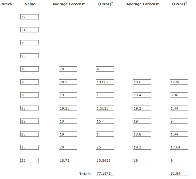
b. Compute the MSE for the four-week and five-week moving average forecasts (to 2 decimals).
| MSE (-Week) | 9.648 |
| MSE (-Week) | 7.406 |
c. What appears to be the best number of weeks of past data (three, four, or five) to use in the moving average computation? Recall that MSE for the three-week moving average is .
The 5-week moving average provides the smallest MSE.
2.Consider the following gasoline time series data. Click on the webfile logo to reference the data.
| Week | Sales (1000s of gallons) | |
| 1 | 17 | |
| 2 | 21 | |
| 3 | 19 | |
| 4 | 23 | |
| 5 | 18 | |
| 6 | 16 | |
| 7 | 20 | |
| 8 | 18 | |
| 9 | 22 | |
| 10 | 20 | |
| 11 | 15 | |
| 12 | 22 | |
a. Applying the MSE measure of forecast accuracy, would you prefer a smoothing constant of or for the gasoline sales time series? Calculate the MSE for each smoothing constant (to 2 decimals).
| MSE for | 9.25 |
| MSE for | 8.98 |
α = 0.2 would be preferred based upon MSE.
b. Are the results the same if you apply MAE as the measure of accuracy? Calculate the MAE (in 1000s of gallons) for each smoothing constant (to 2 decimals).
MAE for 2.57
MAE for 2.59
α = 0.1 would be preferred based upon MAE.
c. What are the results if MAPE is used (to 2 decimals)?
MAPE for 12.95
MAPE for 13.40
α = 0.1 would be preferred based upon MAPE.
3.For the Hawkins Company, the monthly percentages of all shipments received on time over the past months are , , , , , , , , , , , and .
a. Construct a time series plot.
time series plot 3
What type of pattern exists in the data?
horizontal
b. Compare the three-month moving average approach with the exponential smoothing approach for (to 2 decimals). Round intermediate calculations to 2 decimal places.
MSE (-Month) 1.235
MSE () 3.555
4.Which provides more accurate forecasts using MSE as the measure of forecast accuracy?
A 3-months moving average rovides the most accurate forecast using MSE.
c. What is the forecast for next month (to 1 decimal)?
83.33
Ten weeks of data on the Commodity Futures Index are , , , , , , , , , and .
a. Construct a time series plot.
time series plot A
What type of pattern exists in the data?
horizontal
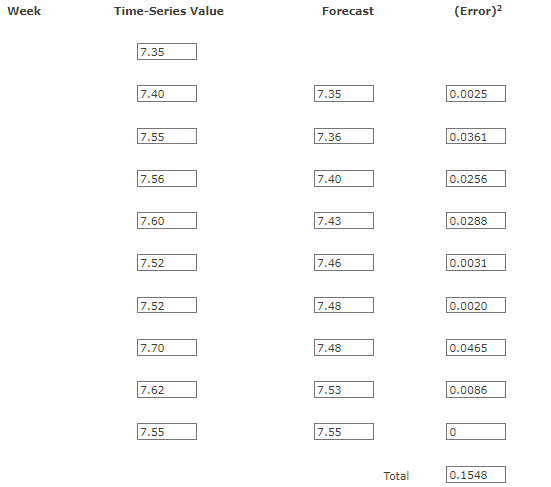
b. Compute the exponential smoothing forecasts for . Round your Time-series values and Forecast values to two decimal places and (Error)2 values to four decimal places.
c. Compute the exponential smoothing forecasts for . Round your Time-series values and Forecast values to two decimal places and (Error)2 values to four decimal places.
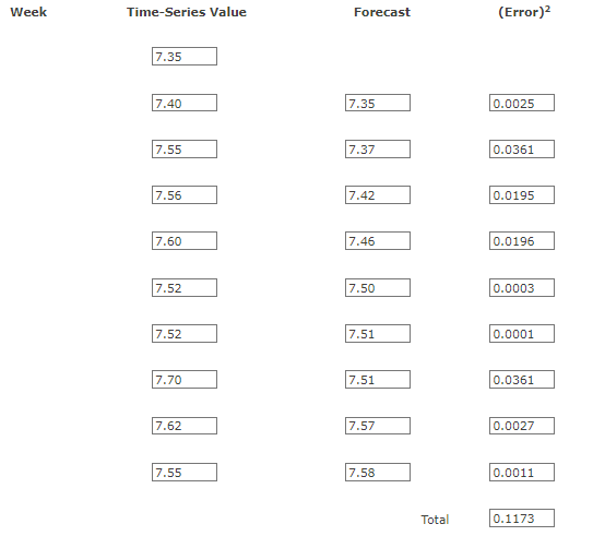
d. Which exponential smoothing constant provides more accurate forecasts based on MSE (to 4 decimals)?
| MSE () | 0.0171 |
| MSE () | 0.0127 |
Forecast week 11 (to 2 decimals).
7.57
5.Consider the following time series.
1 2 3 4 5 6 7
120 110 100 96 94 92 88
a. Construct a time series plot.
time series plot #2
What type of pattern exists in the data?
linear trend
b. Develop the linear trend equation for this time series (to 1 decimal).
119.7 -4.9
c. What is the forecast for (to 1 decimal)?
80.3
6.The following data show the number of Netflix subscribers worldwide for the years (period ) to (period ) (datawrapper website). The data are in the file NetflixSubscribers.
Click on the datafile logo to reference the data.
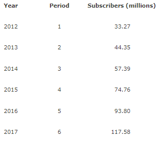
a. Choose the correct time series plot.
Graph C
What type of pattern exists in the data?
Upward
b. Develop a linear trend equation for this time series (to decimals).
16.7791 +11.4647
c. Develop a quadratic trend equation for this time series (to decimals).
1.5625+5.8416+26.048
d. Compare the MSE for each model (to decimals).
| Linear model | 15.30 |
| Quadratic model | 0.11 |
Which model appears better according to MSE?
Quadratic model
e. Use the models developed in parts (b) and (c) to forecast subscribers for (to decimal).
| Linear model | 128.9 |
| Quadratic model | 143.5 |
f. Which of the two forecasts in part (e) would you use? Explain.
For the forecast one period ahead, the Quadratic model is likely slightly preferred because of its Lower MSE
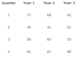
7. Consider the following time series.
a. Construct a time series plot.
plot 1
What type of pattern exists in the data?
Horizontal
b. Use the following dummy variables to develop an estimated regression equation to account for seasonal effects in the data: if Quarter , otherwise; if Quarter , otherwise; if Quarter , otherwise. Enter negative values as negative numbers.
=77+10 Qtr1 + -30 Qtr2 + -20 Qtr3
c. Compute the quarterly forecasts for next year.
| Quarter forecast | 67 |
| Quarter forecast | 47 |
| Quarter forecast | 57 |
| Quarter forecast | 77 |
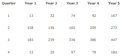
8. South Shore Construction builds permanent docks and seawalls along the southern shore of Long Island, New York. Although the firm has been in business only five years, revenue has increased from in the first year of operation to in the most recent year. The following data show the quarterly sales revenue in thousands of dollars.
a. Construct a time series plot.
Time series plot 2
What type of pattern exists in the data?
There appears to be a seasonal pattern in the data and perhaps a upward linear trend
b. Use the following dummy variables to develop an estimated regression equation to account for any seasonal effects in the data: if Quarter , otherwise; if Quarter , otherwise; if Quarter , otherwise. Round your answers (in thousands of dollars) to whole number.
70.8 4.8 106.4 247.4
Based only on the seasonal effects in the data, compute estimates of quarterly sales for year . Round your answers to whole number.
Quarter forecast $ 75.600 thousands
Quarter forecast $ 177.200 thousands
Quarter forecast $ 318.200 thousands
Quarter forecast $ 70.800 thousands
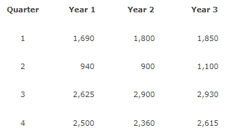
9.The quarterly sales data (number of copies sold) for a college textbook over the past three years follow. Do not round your intermediate calculations.
a. Construct a time series plot.
Time Series plot 1
What type of pattern exists in the data?
linear trend and a seasonal pattern
b. Show the four-quarter and centered moving average values for this time series (to 3 decimals if necessary).
c. Compute the seasonal and adjusted seasonal indexes for the four quarters (to 3 decimals).
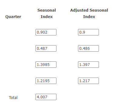
d. When does the publisher have the largest seasonal index?
The largest seasonal index is in the Third quarter.
Does this result appear reasonable?
Yes
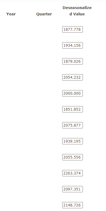
e. Deseasonalize the time series (to 3 decimals).
f. Compute the linear trend equation for the deseasonalized data (to 1 decimal if necessary). Let denote the time series value in ; denote the time series value in ; and so on.
= 1851 + 25.1 Period
Compute the forecast sales using the linear trend equation (to 1 decimal).
| Forecast for quarter | 2177.3 |
| Forecast for quarter | 2202.4 |
| Forecast for quarter | 2227.5 |
| Forecast for quarter | 2252.6 |
g. Adjust the linear trend forecasts using the adjusted seasonal indexes computed in part (c) (to the nearest whole number).
| Forecast for quarter | 1960 |
| Forecast for quarter | 1070 |
| Forecast for quarter | 3112 |
| Forecast for quarter | 2741 |
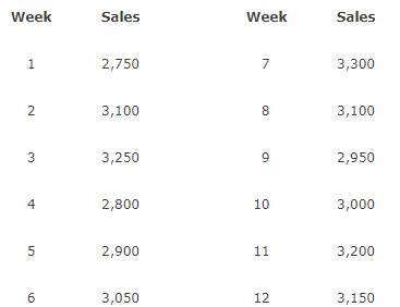
10.United Dairies, Inc., supplies milk to several independent grocers throughout Dade County, Florida. Managers at United Dairies want to develop a forecast of the number of half-gallons of milk sold per week. Sales data for the past weeks follow.
Click on the datafile logo to reference the data.
a. Which of the following time series plots is correct for this data?
time Series plot 2
What type of pattern exists in the data?
horizontal
b. Use exponential smoothing with to develop a forecast of demand for week (to the nearest whole number).
3117 half-gallons of milk
11.Hudson Marine provides boats sales, service, and maintenance. Boat trailers are one of its top sales items. Suppose the quarterly sales values for the seven years of historical data are as follows. Do not round intermediate calculations.
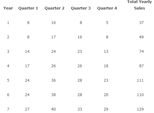
a. Compute the centered moving average values (first find Four-Quarter Moving Average) for this time series (to 3 decimals).
9.25
9.375
10.5
11.875
13
14.625
16.375
17.875
18.875
19.5
20.125
21.125
22.625
24.75
26.25
27.125
27.75
28
28.25
27.875
27.875
28.5
29.375
31.125
b. Choose a time series plot that also shows the centered moving average and original time series on the same graph. Discuss the differences between the original time series plot and the centered moving average time series.
Time Series plot 3
The centered moving average values smooth out the time series by removing seasonal effects
c. Compute the seasonal indexes for the four quarters (to 3 decimals).
Adjusted Seasonal Index
0.872
1.353
1.098
0.678
d. When does Hudson Marine experience the largest seasonal effect?
Hudson Marine experiences the largest seasonal increase in quarter 2 The largest seasonal effect is the seasonal decrease in quarter 4
Does this result seem reasonable?
This is also reasonable because of decreased boating in the fall and winter
CHAPTER 18 ASST
1.The median number of part-time employees at fast-food restaurants in a particular city was known to be last year. City officials think the use of part-time employees may be increasing. A sample of nine fast-food restaurants showed that seven restaurants were employing more than part-time employees, one restaurant was employing exactly part-time employees, and one restaurant was employing fewer than part-time employees. Can it be concluded that the median number of part-time employees has increased? Test using .
Yes
2.Are stock splits beneficial to stockholders? SNL Financial studied stock splits in the banking industry over an -month period. For a sample of stock splits, led to an increase in investment value, led to a decrease in investment value, and resulted in no change. Conduct a sign test to determine if it can be concluded that stock splits are beneficial for holders of bank stocks.
a. What are the null and alternative hypotheses?
Let the probability the shares held will be worth more after the split.
Choose the correct option.
1
b. Using , what is your conclusion?
Conclusion : The results show that stock splits are beneficial to shareholders.
3.A test was conducted for two overnight mail delivery services. Two samples of identical deliveries were set up so that both delivery services were notified of the need for a delivery at the same time. The hours required to make each delivery follow. Do the data shown suggest a difference in the median delivery times for the two services? Use a level of significance for the test. Use Table 1 of Appendix B.
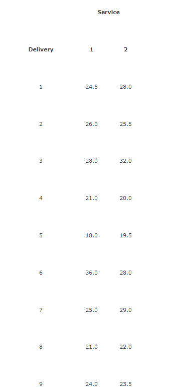
What is the -statistic (to decimals)? Enter negative values as negative number, if necessary.
-0.94
What is the -value (to decimals)?
0.3524
Conclude:
Do not reject the null hypothesis
Observe:
There is not a significant difference.
4.The Scholastic Aptitude Test (SAT) consists of three parts: evidence-based reading, mathematics, and writing. Each part of the test is scored on a – to -point scale with a median of approximately (the College Board website). Scores for each part of the test can be assumed to be symmetric. Use the following data to test the hypothesis that the population median score for the students taking the writing portion of the SAT is . Using , what is your conclusion? Use Table 1 of Appendix B.Click on the datafile logo to reference the data.
Conclusion: We cannot reject the hypothesis that the population median score for the writing portion is 500.
5.Three admission test preparation programs are being evaluated. The scores obtained by a sample of people who used the test preparation programs provided the following data. Use the Kruskal-Wallis test to determine whether there is a significant difference among the three test preparation programs. Use . Use Table 3 of Appendix B.
Click on the datafile logo to reference the data.
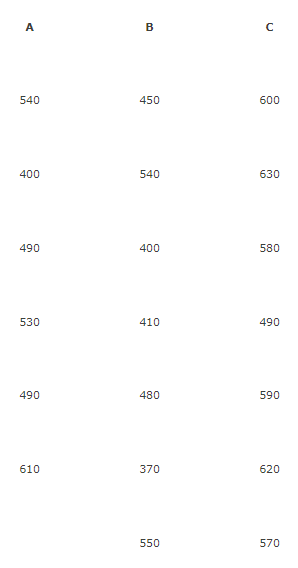
Compute the value of the test statistic (to decimals):
9.06
What is the -value (to decimals)?
0.0106
Conclude:
Reject the null hypothesis
Observe:
We can conclude that there is a significant difference in test preparation programs.
6. The following data show the rankings of states based on expenditure per student (ranked highest to lowest) and student-teacher ratio (ranked lowest to highest). Use Table 1 of Appendix B.
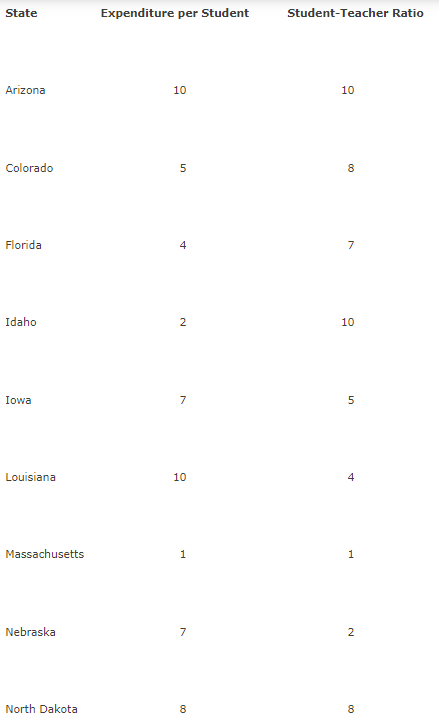
a. What is the rank correlation between expenditure per student and student-teacher ratio (to decimals)? Enter negative values as negative numbers.
-0.05
b. At the level, does there appear to be a relationship between expenditure per student and student-teacher ratio? Enter negative values as negative numbers.
-0.17 (to decimals)
value 0.8631 (to decimals)
we cannot conclude that there is a significant relationship.
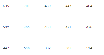
7.A national study by Harris Interactive, Inc., evaluated the top technology companies and their reputations. The following shows how technology companies ranked in reputation and how the companies ranked in percentage of respondents who said they would purchase the company’s stock. A positive rank correlation is anticipated because it seems reasonable to expect that a company with a higher reputation would have the more desirable stock to purchase. Use Table 1 of Appendix B.
Click on the datafile logo to reference the data.
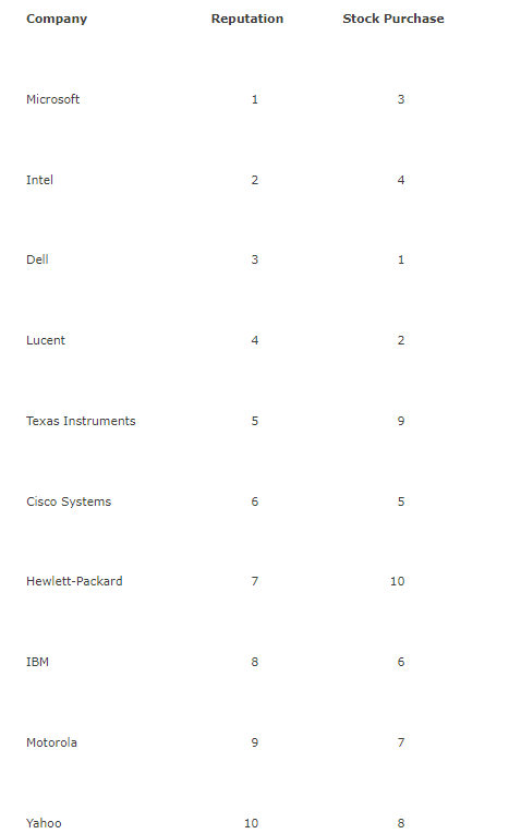
a. Compute the rank correlation between reputation and stock purchase (to decimals).
0.673
b. Test for a significant positive rank correlation.
What is the -statistic (to decimals)?
2.02
What is the -value (to decimals)?
0.0217
c. At , what is your conclusion?
Reject the null hypothesis
Observe:
There is a positive rank correlation.
Other Links:
See other websites for quiz:
Check on QUIZLET