1.Required information
To complete this activity, you will need to have Excel installed on your computer. This exercise requires you to work in Excel and answer questions in Connect. You will read a brief scenario and then download an Excel file that you will need to complete the requirements in Parts 1 through 5 of this exercise. In Part 6, your instructor may require you to upload your completed workbook. Some of the requirements include brief video tutorials on using Excel functions. After viewing the tutorials, you will then use what you learned to work directly in Excel to answer the required questions in Connect.
[The following information applies to the questions displayed below.]
Cary Company manufactures two models of industrial components—a Standard model and an Advanced Model. It has provided the following information with respect to these two products:
| Standard | Advanced | |
|---|---|---|
| Number of units produced and sold | 20,000 | 10,000 |
| Selling price per unit | $ 150 | $ 200 |
| Direct materials per unit | $ 40 | $ 60 |
| Direct labor cost per unit | $ 30 | $ 30 |
| Direct labor-hours per unit | 1.50 | 1.50 |
The company considers all of its manufacturing overhead costs ($1,346,250) to be fixed and it uses plantwide manufacturing overhead cost allocation based on direct labor-hours.
Required:
Click here to download the Excel workbook titled, “ExcelAnalytics_ComparingTraditionalandActivityBasedProductCosting_Template” which you will use to complete the requirements in this exercise.
1. Navigate to the “Plantwide Approach” tab of the Excel workbook. Complete requirements 1a. through 1f. as follows by working directly in Excel and entering your answers in the tabs below.
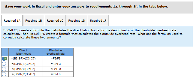
- In Cell F3, create a formula that calculates the direct labor-hours for the denominator of the plantwide overhead rate calculation. Then, in Cell F4, create a formula that calculates the plantwide overhead rate. What are the formulas used to correctly calculate these two amounts?
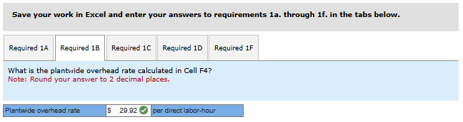
- What is the plantwide overhead rate calculated in Cell F4?
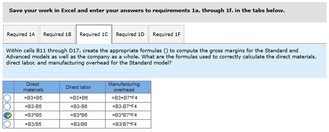
- Within cells B11 through D17, create the appropriate formulas () to compute the gross margins for the Standard and Advanced models as well as the company as a whole. What are the formulas used to correctly calculate the direct materials, direct labor, and manufacturing overhead for the Standard model?
- What are the gross margins for the Standard model calculated in Cell B17and the Advanced model calculated in Cell C17.
- Within the “Plantwide Approach” tab of the Excel workbook, use Charts to create a pie chart that shows the percent of total manufacturing overhead cost allocated to each product using the plantwide approach.
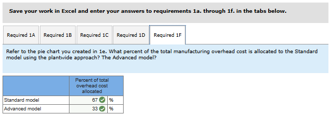
- Refer to the pie chart you created in 1e. What percent of the total manufacturing overhead cost is allocated to the Standard model using the plantwide approach? The Advanced model?

2.Required information
To complete this activity, you will need to have Excel installed on your computer. This exercise requires you to work in Excel and answer questions in Connect. You will read a brief scenario and then download an Excel file that you will need to complete the requirements in Parts 1 through 5 of this exercise. In Part 6, your instructor may require you to upload your completed workbook. Some of the requirements include brief video tutorials on using Excel functions. After viewing the tutorials, you will then use what you learned to work directly in Excel to answer the required questions in Connect.
[The following information applies to the questions displayed below.]
Cary Company manufactures two models of industrial components—a Standard model and an Advanced Model. It has provided the following information with respect to these two products:
| Standard | Advanced | |
|---|---|---|
| Number of units produced and sold | 20,000 | 10,000 |
| Selling price per unit | $ 150 | $ 200 |
| Direct materials per unit | $ 40 | $ 60 |
| Direct labor cost per unit | $ 30 | $ 30 |
| Direct labor-hours per unit | 1.50 | 1.50 |
The company considers all of its manufacturing overhead costs ($1,346,250) to be fixed and it uses plantwide manufacturing overhead cost allocation based on direct labor-hours.
Cary’s production manager has suggested replacing the company’s current cost system with an activity-based costing system that assigns all of the company’s manufacturing overhead costs to four activity cost pools as follows (the company does not have any organization-sustaining costs or unused capacity costs):
| Activity Measure | Activity Measure | Manufacturing Overhead |
|---|---|---|
| Assemble and pack | Direct labor hours | $ 292,500 |
| Machining | Machine-hours | 440,000 |
| Order processing | Number of customer orders | 256,250 |
| Setups | Setup hours | 357,500 |
| $ 1,346,250 |
The production manager also provided the following additional information with respect to the company’s two products:
| Standard | Advanced | |
|---|---|---|
| Machine-hours per unit | 1.0 | 2.0 |
| Average customer order size (in units) | 400 | 50 |
| Number of setups per customer order | 1 | 1 |
| Number of setup hours per setup | 1 | 3 |
Use the Excel workbook titled “ExcelAnalytics_ComparingTraditionalandActivityBasedProductCosting_Template” to complete requirements 2a. and 2b.
- 2a. Navigate to the “Activity Based Approach.” tab of the Excel workbook. Within the Activity Rates section of this tab, create formulas that calculate the activity rates in cells G5, G10, G15, and G20.
- 2b. On the table below, enter the activity rate for each of the four activities as calculated by the formulas you created in requirement 2a.
Note: Round your answers to 2 decimal places.

3.Required information
To complete this activity, you will need to have Excel installed on your computer. This exercise requires you to work in Excel and answer questions in Connect. You will read a brief scenario and then download an Excel file that you will need to complete the requirements in Parts 1 through 5 of this exercise. In Part 6, your instructor may require you to upload your completed workbook. Some of the requirements include brief video tutorials on using Excel functions. After viewing the tutorials, you will then use what you learned to work directly in Excel to answer the required questions in Connect.
[The following information applies to the questions displayed below.]
Cary Company manufactures two models of industrial components—a Standard model and an Advanced Model. It has provided the following information with respect to these two products:
| Standard | Advanced | |
|---|---|---|
| Number of units produced and sold | 20,000 | 10,000 |
| Selling price per unit | $ 150 | $ 200 |
| Direct materials per unit | $ 40 | $ 60 |
| Direct labor cost per unit | $ 30 | $ 30 |
| Direct labor-hours per unit | 1.50 | 1.50 |
The company considers all of its manufacturing overhead costs ($1,346,250) to be fixed and it uses plantwide manufacturing overhead cost allocation based on direct labor-hours.
Use the Excel workbook titled “ExcelAnalytics_ComparingTraditionalandActivityBasedProductCosting_Template” to complete requirements 3a. through 3c.
3. Navigate to the “Activity Based Approach” tab of the Excel workbook and go to the section called “Product Margin Analysis.” Within cells B16 through C19, create formulas that calculate the amounts of overhead cost that should be allocated from each activity cost pool to each product. Also, in cells B21 through D21, create all of the formulas necessary to compute the product margins for each product, and for the company as a whole.
- What are the formulas used in cells C18 and C19 to correctly calculate the cost assignments for the Advanced model from the Order Processing and Setups activities?
- How much overhead cost is assigned from each of the four activities to the Standard and Advanced models?
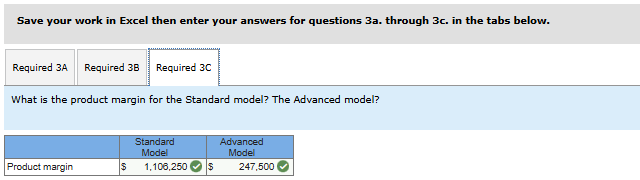
- What is the product margin for the Standard model? The Advanced model?


4.Required information
To complete this activity, you will need to have Excel installed on your computer. This exercise requires you to work in Excel and answer questions in Connect. You will read a brief scenario and then download an Excel file that you will need to complete the requirements in Parts 1 through 7 of this exercise.
Some of the requirements include brief video tutorials on using Excel functions. After viewing the tutorials, you will then use what you learned to work directly in Excel to answer the required questions in Connect.
[The following information applies to the questions displayed below.]
Lyndia Company is a merchandiser that sells a total of 15 products to its customers. The company provided the following information from last year:
| Product | Unit Sales | Selling Price per Unit | Variable Cost per Unit |
|---|---|---|---|
| 1 | 9,000 | $ 29 | $ 12.95 |
| 2 | 16,500 | $ 99 | $ 68.55 |
| 3 | 6,000 | $ 85 | $ 42.50 |
| 4 | 19,500 | $ 109 | $ 85.00 |
| 5 | 4,500 | $ 19 | $ 6.35 |
| 6 | 27,000 | $ 119 | $ 92.00 |
| 7 | 3,000 | $ 39 | $ 14.30 |
| 8 | 7,500 | $ 79 | $ 33.18 |
| 9 | 9,000 | $ 69 | $ 30.36 |
| 10 | 15,000 | $ 95 | $ 77.60 |
| 11 | 10,500 | $ 59 | $ 25.40 |
| 12 | 1,500 | $ 65 | $ 29.00 |
| 13 | 3,000 | $ 44 | $ 12.40 |
| 14 | 6,000 | $ 49 | $ 13.48 |
| 15 | 12,000 | $ 89 | $ 61.83 |
| 150,000 |
Last year, Lyndia’s total fixed expenses and net operating income were $3,000,000 and $1,223,070, respectively. The company would like your assistance in developing some financial projections for this year.
Required:
Click here to download the Excel workbook titled “ExcelAnalytics_CVPRelationships2_Template”.
1. To confirm your understanding of the spreadsheet’s design, navigate to the “Requirement 1” tab of the Excel workbook and answer the following questions with respect to last year:
- How is the percentage in cell B3 calculated? Why do you think specifying the sales mix percentages for all products is important?
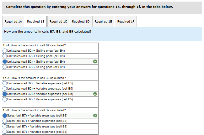
- How are the amounts in cells B7, B8, and B9 calculated?
- How are the amounts in cells Q7, Q8, and Q9 calculated?
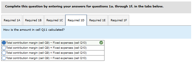
- How is the amount in cell Q11 calculated?
- How are the percentages in cells R8 and R9 calculated?
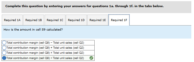
- How is the amount in cell S9 calculated?


5.Required information
To complete this activity, you will need to have Excel installed on your computer. This exercise requires you to work in Excel and answer questions in Connect. You will read a brief scenario and then download an Excel file that you will need to complete the requirements in Parts 1 through 7 of this exercise.
Some of the requirements include brief video tutorials on using Excel functions. After viewing the tutorials, you will then use what you learned to work directly in Excel to answer the required questions in Connect.
[The following information applies to the questions displayed below.]
Lyndia Company is a merchandiser that sells a total of 15 products to its customers. The company provided the following information from last year:
| Product | Unit Sales | Selling Price per Unit | Variable Cost per Unit |
|---|---|---|---|
| 1 | 9,000 | $ 29 | $ 12.95 |
| 2 | 16,500 | $ 99 | $ 68.55 |
| 3 | 6,000 | $ 85 | $ 42.50 |
| 4 | 19,500 | $ 109 | $ 85.00 |
| 5 | 4,500 | $ 19 | $ 6.35 |
| 6 | 27,000 | $ 119 | $ 92.00 |
| 7 | 3,000 | $ 39 | $ 14.30 |
| 8 | 7,500 | $ 79 | $ 33.18 |
| 9 | 9,000 | $ 69 | $ 30.36 |
| 10 | 15,000 | $ 95 | $ 77.60 |
| 11 | 10,500 | $ 59 | $ 25.40 |
| 12 | 1,500 | $ 65 | $ 29.00 |
| 13 | 3,000 | $ 44 | $ 12.40 |
| 14 | 6,000 | $ 49 | $ 13.48 |
| 15 | 12,000 | $ 89 | $ 61.83 |
| 150,000 |
Last year, Lyndia’s total fixed expenses and net operating income were $3,000,000 and $1,223,070, respectively. The company would like your assistance in developing some financial projections for this year.
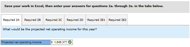
2. Navigate to the “Requirement 2” tab of the Excel workbook. Regarding projections for this year, assume that total unit sales increase by 10%, and everything else holds constant. (Hint: The template contains dynamic formulas, therefore you will only need to modify the input in cell Q15 to complete requirements 2a through 2e.)
- What would be the projected net operating income for this year?
- How are the projected unit sales in cells B22 and Q22 calculated?
- Why are the percentages in cells R28 and R29 the same as the corresponding percentages in cells R8 and R9 even though the projected sales of 165,000 units is 15,000 units greater than last year’s sales of 150,0000 units?
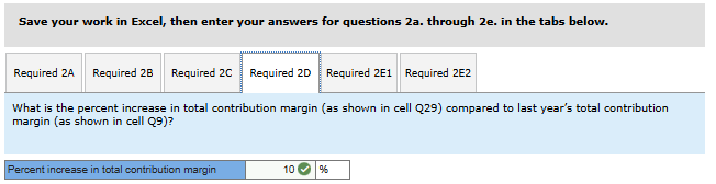
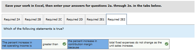
- What is the percent increase in total contribution margin (as shown in cell Q29) compared to last year’s total contribution margin (as shown in cell Q9)?
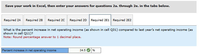
- What is the percent increase in net operating income (as shown in cell Q31) compared to last year’s net operating income (as shown in cell Q11)? Is your answer greater than, less than, or equal to your answer in requirement 2d?


6.Required information
To complete this activity, you will need to have Excel installed on your computer. This exercise requires you to work in Excel and answer questions in Connect. You will read a brief scenario and then download an Excel file that you will need to complete the requirements in Parts 1 and 2 of this exercise.
Some of the requirements include brief video tutorials on using Excel functions. After viewing the tutorials, you will then use what you learned to work directly in Excel to answer the required questions in Connect.
[The following information applies to the questions displayed below.]
Williams Company’s accounting department has finished preparing the master budget for this year. The chief financial officer (CFO) would like your assistance in creating data visualizations that she can use to better explain the master budget to the company’s senior management team.
You decide to break down your assignment into two parts. First, you will review the master budget to ensure that you understand all of its schedules and their interrelationships. Second, you will prepare the data visualizations that have been requested by the CFO.
Required:
To improve your understanding of all schedules included in the master budget and their interrelationships, refer to the Excel workbook and answer the following questions:
- Go to the “Sales Budget” tab:
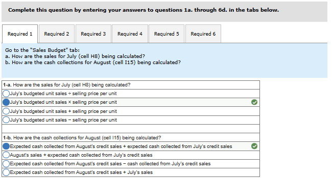
- How are the sales for July (cell H8) being calculated?
- How are the cash collections for August (cell I15) being calculated?
- Go to the “Merchandise Purchases Budget” tab:
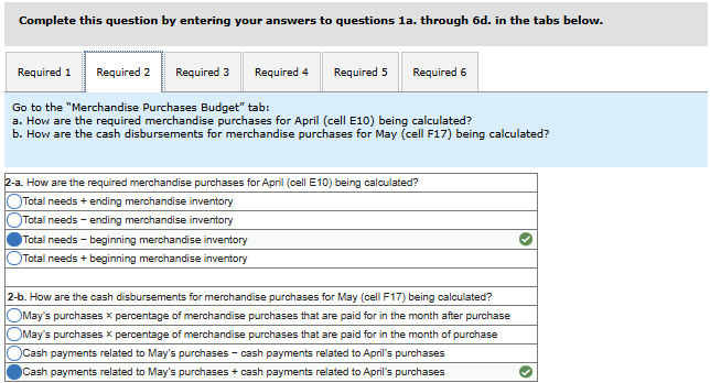
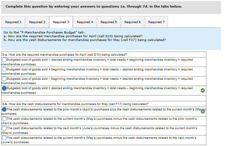
- How are the required merchandise purchases for April (cell E10) being calculated?
- How are the cash disbursements for merchandise purchases for May (cell F17) being calculated?
- Go to the “Selling & Admin Budget” tab:
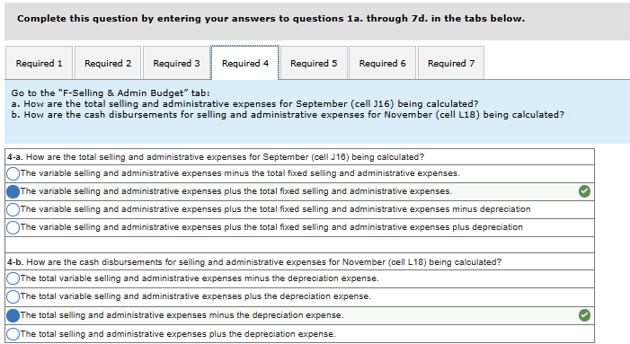
- How are the total selling and administrative expenses for September (cell J16) being calculated?
- How are the cash disbursements for selling and administrative expenses for November (cell L18) being calculated?
- Go to the “Cash Budget” tab:
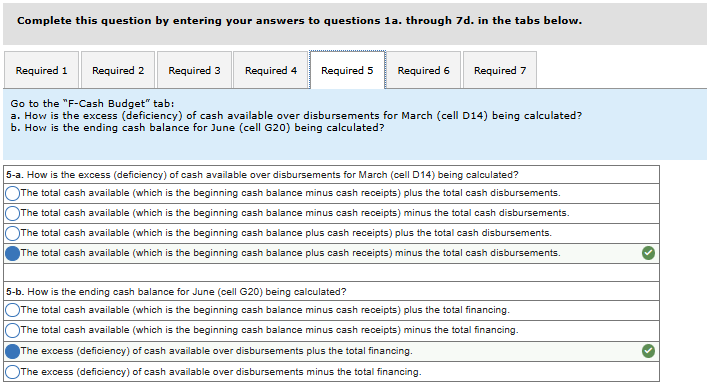
- How is the excess (deficiency) of cash available over disbursements for March (cell D14) being calculated?
- How is the ending cash balance for June (cell G20) being calculated?
- Go to the “Budgeted Income Statements” tab:
- How is the cost of goods sold for February (cell C8) being calculated?
- How is the net income for April (cell E13) being calculated?
- Go to the “Budgeted Balance Sheets” tab:
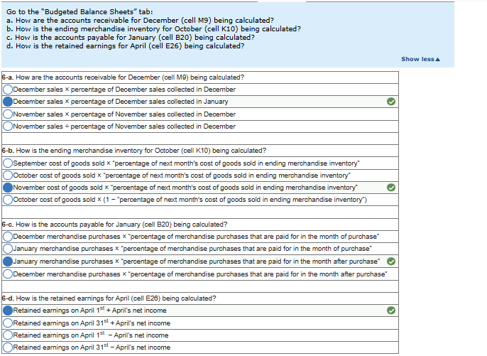
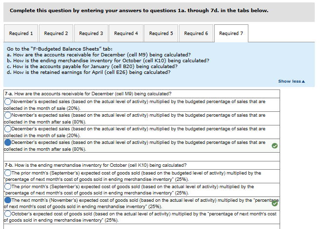
- How are the accounts receivable for December (cell M9) being calculated?
- How is the ending merchandise inventory for October (cell K10) being calculated?
- How is the accounts payable for January (cell B20) being calculated?
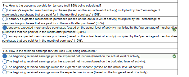
- How is the retained earnings for April (cell E26) being calculated?


7.Required information
To complete this activity, you will need to have Excel installed on your computer. This exercise requires you to work in Excel and answer questions in Connect. You will read a brief scenario and then download an Excel file that you will need to complete the requirements in Parts 1 and 2 of this exercise.
Some of the requirements include brief video tutorials on using Excel functions. After viewing the tutorials, you will then use what you learned to work directly in Excel to answer the required questions in Connect.
[The following information applies to the questions displayed below.]
Williams Company’s accounting department has finished preparing the master budget for this year. The chief financial officer (CFO) would like your assistance in creating data visualizations that she can use to better explain the master budget to the company’s senior management team.
You decide to break down your assignment into two parts. First, you will review the master budget to ensure that you understand all of its schedules and their interrelationships. Second, you will prepare the data visualizations that have been requested by the CFO.
Click here for a brief tutorial on using Charts in Excel.
Use the Excel workbook titled, “ExcelAnalytics_MasterBudgeting_Template” to complete requirements 7 and 8.
- The CFO would like you to prepare some data visualizations that depict trends in sales, net income, and cash collections. Accordingly, use Charts to do the following:Note: For the questions displayed below, you may select more than one answer. Single click the box with the question mark to produce a check mark for a correct answer or double click the box with the question mark to empty the box for a wrong answer. Boxes left with a question mark will be automatically graded as incorrect.
- Within the “Sales Budget” tab of the Excel workbook, create a line chart that provides a monthly sales trend analysis.
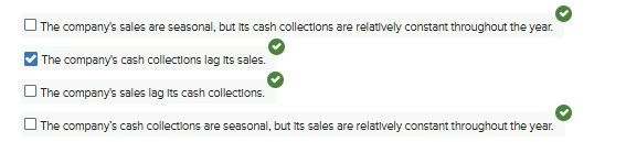
- Which of the following statements are true based on the line chart that you created in requirement 7a?

- Within the “Sales Budget” tab of the Excel workbook, create a line chart that includes the monthly sales trend analysis from requirement 7a plus another trend line pertaining to the monthly cash collections from customers.
- Which of the following statements are true based on the line chart that you created in requirement 7c?
- Within the “Budgeted Income Statements” tab of the Excel workbook, create a line chart that includes the monthly sales trend analysis from requirement 7a plus another trend line pertaining to monthly net income.
- Which of the following statements are true based on the line chart that you created in requirement 7e?

The CFO would also like you to prepare some data visualizations that depict monthly trends in the cash balance, current assets, and net income. Accordingly, use Charts to do the following:
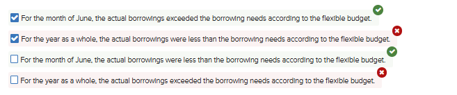
- Within the “Cash Budget” tab of the Excel workbook, create a bar chart that includes one bar for each of 12 months. Each month’s bar will show the excess (deficiency) of cash available over disbursements for that month and (where appropriate) the borrowings for that month. Use different colors to distinguish the excess (deficiency) of cash available over disbursements from any borrowings. Also, insert a horizontal line within your chart to depict the company’s minimum cash balance of $30,000.
- Which of the following statements are true based on the bar chart that you created in requirement 8a?

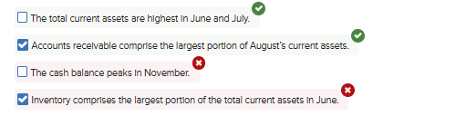
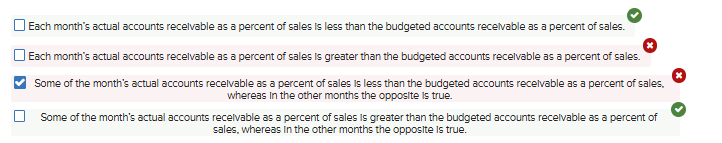
- Within the “Budgeted Balance Sheets” tab of the Excel workbook, create a bar chart that depicts each month’s ending total current assets. Each bar within the chart will sub-divide into three parts to represent the portion of the overall balance that resides in cash, accounts receivable, and inventory.
- Which of the following statements are true based on the bar chart that you created in requirement 8c?
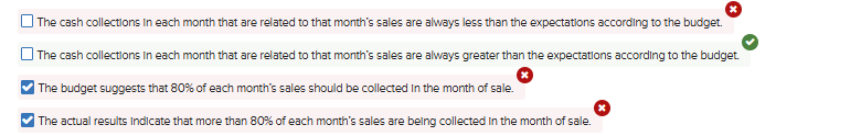
- Go to the “Cash Flow vs. Net Income” tab and create a line chart that includes a total of two lines. The first line will depict monthly trends in operating cash flows (cash collections from customers minus total cash disbursements, including interest payments) and the second line will depict net income.
- Which of the following statements are true based on the line chart that you created in requirement 8e?

8.Required information
To complete this activity, you will need to have Excel installed on your computer. This exercise requires you to work in Excel and answer questions in Connect. You will read a brief scenario and then download an Excel file that you will need to complete the requirements in Parts 1 through 3 of this exercise.
Some of the requirements include brief video tutorials on using Excel functions. After viewing the tutorials, you will then use what you learned to work directly in Excel to answer the required questions in Connect.
[The following information applies to the questions displayed below.]
Williams Company’s accounting department has finished preparing a flexible budget to better understand the differences between its actual results and the master budget. The chief financial officer (CFO) would like your assistance in creating data visualizations that she can use to explain why the company’s actual results differed from its master budget.
You decide to break down your assignment into two parts. First, you will review the flexible budget to ensure that you understand all of its schedules and their interrelationships as well as how it differs from the master budget. Second, you will prepare the data visualizations that have been requested by the CFO.
Required:
To improve your understanding of all the schedules included in the flexible budget and their relationship to the master budget, refer to the Excel workbook and answer the following questions:
- Review the “M-Budgeting Assumptions” and “F-Budgeting Assumptions” tabs:
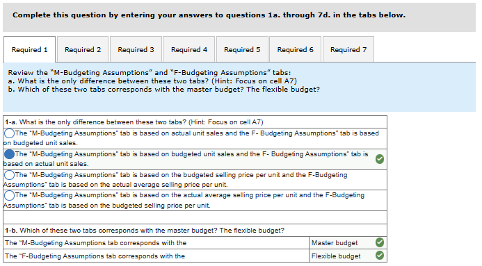
- What is the only difference between these two tabs? (Hint: Focus on cell A7)
- Which of these two tabs corresponds with the master budget? The flexible budget?
- Go to the “F-Sales Budget” tab:
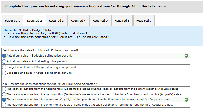
- How are the sales for July (cell H8) being calculated?
- How are the cash collections for August (cell I15) being calculated?
- Go to the “F-Merchandise Purchases Budget” tab:
- How are the required merchandise purchases for April (cell E10) being calculated?
- How are the cash disbursements for merchandise purchases for May (cell F17) being calculated?
- Go to the “F-Selling & Admin Budget” tab:
- How are the total selling and administrative expenses for September (cell J16) being calculated?
- How are the cash disbursements for selling and administrative expenses for November (cell L18) being calculated?
- Go to the “F-Cash Budget” tab:
- How is the excess (deficiency) of cash available over disbursements for March (cell D14) being calculated?
- How is the ending cash balance for June (cell G20) being calculated?
- Go to the “F-Budgeted Income Statements” tab:
- How is the cost of goods sold for February (cell C8) being calculated?
- How is the net income for April (cell E13) being calculated?
- Go to the “F-Budgeted Balance Sheets” tab:
- How are the accounts receivable for December (cell M9) being calculated?
- How is the ending merchandise inventory for October (cell K10) being calculated?
- How is the accounts payable for January (cell B20) being calculated?
- How is the retained earnings for April (cell E26) being calculated?

9.Required information
To complete this activity, you will need to have Excel installed on your computer. This exercise requires you to work in Excel and answer questions in Connect. You will read a brief scenario and then download an Excel file that you will need to complete the requirements in Parts 1 through 3 of this exercise.
Some of the requirements include brief video tutorials on using Excel functions. After viewing the tutorials, you will then use what you learned to work directly in Excel to answer the required questions in Connect.
[The following information applies to the questions displayed below.]
Williams Company’s accounting department has finished preparing a flexible budget to better understand the differences between its actual results and the master budget. The chief financial officer (CFO) would like your assistance in creating data visualizations that she can use to explain why the company’s actual results differed from its master budget.
You decide to break down your assignment into two parts. First, you will review the flexible budget to ensure that you understand all of its schedules and their interrelationships as well as how it differs from the master budget. Second, you will prepare the data visualizations that have been requested by the CFO.
Continue using the Excel workbook, “ExcelAnalytics_FlexibleBudgetingandFSA_Template” to complete Part 2.
Based on the charts you prepared in Part 2 answer the following questions:
Note: Note that for all questions below you may select more than one answer. Single click the box with the question mark to produce a check mark for a correct answer or double click the box with the question mark to empty the box for a wrong answer. Any boxes left with a question mark will be automatically graded as incorrect.
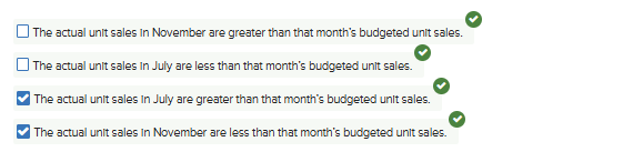
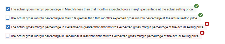
1.Based on a review of the Sales Analysis from Part 2 Requirement 8a, which of the following statements are true?
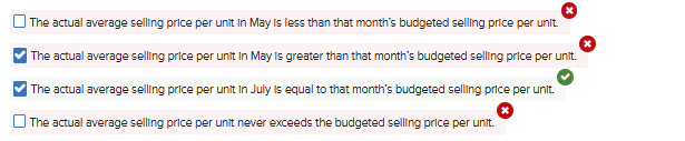
2.Based on a review of the Sales Analysis from Part 2 Requirement 8a, which of the following statements are true?
3.Based on a review of the Gross Margin Analysis from Part 2 Requirement 8b, which of the following statements are true?
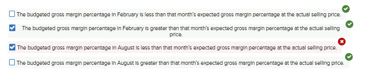
4.Based on a review of the Gross Margin Analysis from Part 2 Requirement 8b, which of the following statements are true?
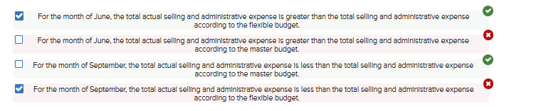
5.Based on a review of the Selling and Administrative Expense Analysis from Part 2 Requirement 8c, which of the following statements are true?

6.Based on a review of the Selling and Administrative Expense Analysis from Part 2 Requirement 8c, which of the following statements are true?
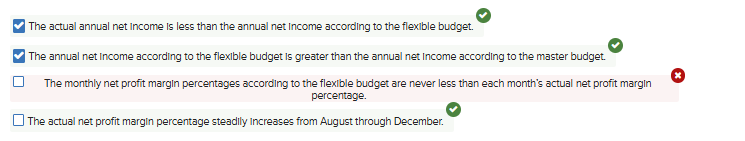
7.Based on a review of the Profit Analysis from Part 2 Requirement 8d, which of the following statements are true?
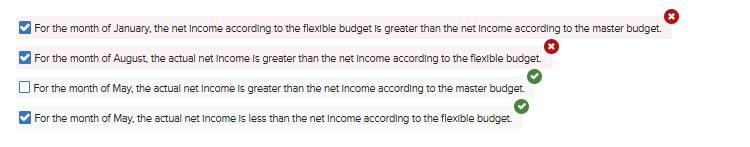
8.Based on a review of the Profit Analysis from Part 2 Requirement 8d, which of the following statements are true?
9.Based on a review of the Cumulative Operating Cash Flow Analysis from Part 2 Requirement 9a, which of the following statements are true?

10.Based on a review of the Cumulative Operating Cash Flow Analysis from Part 2 Requirement 9a, which of the following statements are true?

11.Based on a review of the Financing Analysis from Part 2 Requirement 9b, which of the following statements are true?

12.Based on a review of the Financing Analysis from Part 2 Requirement 9b, which of the following statements are true?
13.Based on a review of the Accounts Receivable Analysis from Part 2 Requirement 9c, which of the following statements are true?
14.Based on a review of the Accounts Receivable Analysis from Part 2 Requirement 9c, which of the following statements are true?
10.Required information
TTo complete this activity, you will need to have Excel installed on your computer. This exercise requires you to work in Excel and answer questions in Connect. You will read a brief scenario and then download an Excel file that you will need to complete the requirements in Parts 1 through 9b of this exercise.
TSome of the requirements include brief video tutorials on using Excel functions. After viewing the tutorials, you will then use what you learned to work directly in Excel to answer the required questions in Connect.
[The following information applies to the questions displayed below.]
Edman Company is a merchandiser that has provided the following balance sheet and income statement for this year.
| Beginning Balance | Ending Balance | |
|---|---|---|
| Assets | ||
| Cash | $62,800 | $150,000 |
| Accounts receivable | 160,000 | 180,000 |
| Inventory | 230,000 | 240,000 |
| Property, plant & equipment (net) | 833,000 | 793,000 |
| Other assets | 37,000 | 37,000 |
| Total assets | $1,322,800 | $1,400,000 |
| Liabilities & Stockholders’ Equity | ||
| Accounts payable | $70,000 | $80,000 |
| Bonds payable | 550,000 | 550,000 |
| Common stock | 410,000 | 410,000 |
| Retained earnings | 292,800 | 360,000 |
| Total liabilities & stockholders’ equity | $1,322,800 | $1,400,000 |
| This Year | |
|---|---|
| Sales | $2,500,000 |
| Variable expenses: | |
| Cost of goods sold | 1,600,000 |
| Variable selling expense | 240,000 |
| Total variable expenses | 1,840,000 |
| Contribution margin | 660,000 |
| Fixed expenses: | |
| Fixed selling expenses | 220,000 |
| Fixed administrative expenses | 300,000 |
| Total fixed expenses | 520,000 |
| Net operating income | 140,000 |
| Interest expense (8%) | 44,000 |
| Net income before tax | 96,000 |
| Tax expense (30%) | 28,800 |
| Net income | $67,200 |
Required:
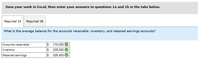
1. Refer to the “Requirement 1 Financials” tab within your Excel workbook. For this year, create formulas within column D that calculate the average balance for each balance sheet account.
- What is the average balance for the accounts receivable, inventory, and retained earnings accounts?
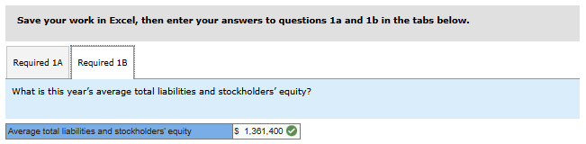
- What is this year’s average total liabilities and stockholders’ equity?
11.Required information
TTo complete this activity, you will need to have Excel installed on your computer. This exercise requires you to work in Excel and answer questions in Connect. You will read a brief scenario and then download an Excel file that you will need to complete the requirements in Parts 1 through 9b of this exercise.
TSome of the requirements include brief video tutorials on using Excel functions. After viewing the tutorials, you will then use what you learned to work directly in Excel to answer the required questions in Connect.
[The following information applies to the questions displayed below.]
Edman Company is a merchandiser that has provided the following balance sheet and income statement for this year.
| Beginning Balance | Ending Balance | |
|---|---|---|
| Assets | ||
| Cash | $62,800 | $150,000 |
| Accounts receivable | 160,000 | 180,000 |
| Inventory | 230,000 | 240,000 |
| Property, plant & equipment (net) | 833,000 | 793,000 |
| Other assets | 37,000 | 37,000 |
| Total assets | $1,322,800 | $1,400,000 |
| Liabilities & Stockholders’ Equity | ||
| Accounts payable | $70,000 | $80,000 |
| Bonds payable | 550,000 | 550,000 |
| Common stock | 410,000 | 410,000 |
| Retained earnings | 292,800 | 360,000 |
| Total liabilities & stockholders’ equity | $1,322,800 | $1,400,000 |
| This Year | |
|---|---|
| Sales | $2,500,000 |
| Variable expenses: | |
| Cost of goods sold | 1,600,000 |
| Variable selling expense | 240,000 |
| Total variable expenses | 1,840,000 |
| Contribution margin | 660,000 |
| Fixed expenses: | |
| Fixed selling expenses | 220,000 |
| Fixed administrative expenses | 300,000 |
| Total fixed expenses | 520,000 |
| Net operating income | 140,000 |
| Interest expense (8%) | 44,000 |
| Net income before tax | 96,000 |
| Tax expense (30%) | 28,800 |
| Net income | $67,200 |
2. Refer to the “Requirement 2 DuPont Diagram” tab within your Excel workbook. For this year, complete the diagram by using appropriate formulas and reference cells. (In some instances your formulas and reference cells will refer to the Requirement 1 Financials tab.)
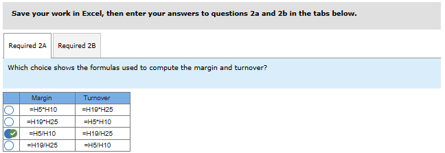
- Which choice shows the formulas used to compute the margin and turnover?
- What is this year’s margin, turnover, and return on investment (ROI)?
For next year, the company is interested in pursuing one of three proposed courses of action. Each of these three alternatives will be independently evaluated in subsequent requirements.

12.Required information
TTo complete this activity, you will need to have Excel installed on your computer. This exercise requires you to work in Excel and answer questions in Connect. You will read a brief scenario and then download an Excel file that you will need to complete the requirements in Parts 1 through 9b of this exercise.
TSome of the requirements include brief video tutorials on using Excel functions. After viewing the tutorials, you will then use what you learned to work directly in Excel to answer the required questions in Connect.
[The following information applies to the questions displayed below.]
Edman Company is a merchandiser that has provided the following balance sheet and income statement for this year.
| Beginning Balance | Ending Balance | |
|---|---|---|
| Assets | ||
| Cash | $62,800 | $150,000 |
| Accounts receivable | 160,000 | 180,000 |
| Inventory | 230,000 | 240,000 |
| Property, plant & equipment (net) | 833,000 | 793,000 |
| Other assets | 37,000 | 37,000 |
| Total assets | $1,322,800 | $1,400,000 |
| Liabilities & Stockholders’ Equity | ||
| Accounts payable | $70,000 | $80,000 |
| Bonds payable | 550,000 | 550,000 |
| Common stock | 410,000 | 410,000 |
| Retained earnings | 292,800 | 360,000 |
| Total liabilities & stockholders’ equity | $1,322,800 | $1,400,000 |
| This Year | |
|---|---|
| Sales | $2,500,000 |
| Variable expenses: | |
| Cost of goods sold | 1,600,000 |
| Variable selling expense | 240,000 |
| Total variable expenses | 1,840,000 |
| Contribution margin | 660,000 |
| Fixed expenses: | |
| Fixed selling expenses | 220,000 |
| Fixed administrative expenses | 300,000 |
| Total fixed expenses | 520,000 |
| Net operating income | 140,000 |
| Interest expense (8%) | 44,000 |
| Net income before tax | 96,000 |
| Tax expense (30%) | 28,800 |
| Net income | $67,200 |
3. To evaluate alternative 1 of the proposed actions for next year, refer to the “Requirement 3 Financials” tab within your Excel workbook. Assume the company streamlines it working capital management practices with the following estimated impacts:
- Next year’s ending balance in accounts receivable decreases by $80,000 compared to its beginning balance.
- Next year’s ending balance in inventory decreases by $120,000 compared to its beginning balance.
- Next year’s ending balance in property, plant, and equipment (net) decreases by $40,000 compared to its beginning balance to reflect next year’s depreciation expense.
- Next year’s ending balance in accounts payable decreases by $40,000 compared to its beginning balance.
- Next year’s ending balance in bonds payable decreases by $300,000 compared to its beginning balance to reflect a retirement of bonds payable.
- Next year’s ending balances in other assets and common stock are the same as their beginning balances.
- Next year’s total sales, variables expenses, fixed expenses, and net operating income are the same as this year.
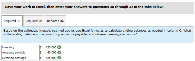
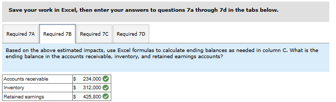
- Based on the estimated impacts outlined above, use Excel formulas to calculate ending balances as needed in column C. What is the ending balance in the inventory, accounts payable, and retained earnings accounts?
- Create formulas within column D that calculate next year’s average balances for all balance sheet accounts (except Cash which will automatically be computed for you). What is the average balance in the inventory, accounts payable, and retained earnings accounts?
- What is the company’s estimated average total liabilities and stockholders’ equity for next year?


13.Required information
TTo complete this activity, you will need to have Excel installed on your computer. This exercise requires you to work in Excel and answer questions in Connect. You will read a brief scenario and then download an Excel file that you will need to complete the requirements in Parts 1 through 9b of this exercise.
TSome of the requirements include brief video tutorials on using Excel functions. After viewing the tutorials, you will then use what you learned to work directly in Excel to answer the required questions in Connect.
[The following information applies to the questions displayed below.]
Edman Company is a merchandiser that has provided the following balance sheet and income statement for this year.
| Beginning Balance | Ending Balance | |
|---|---|---|
| Assets | ||
| Cash | $62,800 | $150,000 |
| Accounts receivable | 160,000 | 180,000 |
| Inventory | 230,000 | 240,000 |
| Property, plant & equipment (net) | 833,000 | 793,000 |
| Other assets | 37,000 | 37,000 |
| Total assets | $1,322,800 | $1,400,000 |
| Liabilities & Stockholders’ Equity | ||
| Accounts payable | $70,000 | $80,000 |
| Bonds payable | 550,000 | 550,000 |
| Common stock | 410,000 | 410,000 |
| Retained earnings | 292,800 | 360,000 |
| Total liabilities & stockholders’ equity | $1,322,800 | $1,400,000 |
| This Year | |
|---|---|
| Sales | $2,500,000 |
| Variable expenses: | |
| Cost of goods sold | 1,600,000 |
| Variable selling expense | 240,000 |
| Total variable expenses | 1,840,000 |
| Contribution margin | 660,000 |
| Fixed expenses: | |
| Fixed selling expenses | 220,000 |
| Fixed administrative expenses | 300,000 |
| Total fixed expenses | 520,000 |
| Net operating income | 140,000 |
| Interest expense (8%) | 44,000 |
| Net income before tax | 96,000 |
| Tax expense (30%) | 28,800 |
| Net income | $67,200 |
4. Refer to the “Requirement 4 DuPont Diagram” tab within your Excel workbook. For alternative 1, complete the diagram by using appropriate formulas and reference cells. (In some instances your formulas and reference cells will refer to the “Requirement 3 Financials” tab.)
- Which choice shows the formulas used to compute the net operating income and average operating assets?
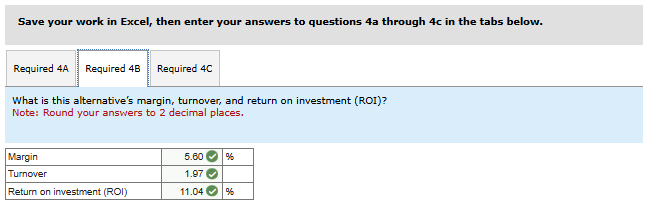
- What is this alternative’s margin, turnover, and return on investment (ROI)?
- If the company pursues this alternative, would it cause next year’s ROI to be greater than, less than, or equal to this year’s ROI (as computed in Requirement 2b)?


14.Required information
TTo complete this activity, you will need to have Excel installed on your computer. This exercise requires you to work in Excel and answer questions in Connect. You will read a brief scenario and then download an Excel file that you will need to complete the requirements in Parts 1 through 9b of this exercise.
TSome of the requirements include brief video tutorials on using Excel functions. After viewing the tutorials, you will then use what you learned to work directly in Excel to answer the required questions in Connect.
[The following information applies to the questions displayed below.]
Edman Company is a merchandiser that has provided the following balance sheet and income statement for this year.
| Beginning Balance | Ending Balance | |
|---|---|---|
| Assets | ||
| Cash | $62,800 | $150,000 |
| Accounts receivable | 160,000 | 180,000 |
| Inventory | 230,000 | 240,000 |
| Property, plant & equipment (net) | 833,000 | 793,000 |
| Other assets | 37,000 | 37,000 |
| Total assets | $1,322,800 | $1,400,000 |
| Liabilities & Stockholders’ Equity | ||
| Accounts payable | $70,000 | $80,000 |
| Bonds payable | 550,000 | 550,000 |
| Common stock | 410,000 | 410,000 |
| Retained earnings | 292,800 | 360,000 |
| Total liabilities & stockholders’ equity | $1,322,800 | $1,400,000 |
| This Year | |
|---|---|
| Sales | $2,500,000 |
| Variable expenses: | |
| Cost of goods sold | 1,600,000 |
| Variable selling expense | 240,000 |
| Total variable expenses | 1,840,000 |
| Contribution margin | 660,000 |
| Fixed expenses: | |
| Fixed selling expenses | 220,000 |
| Fixed administrative expenses | 300,000 |
| Total fixed expenses | 520,000 |
| Net operating income | 140,000 |
| Interest expense (8%) | 44,000 |
| Net income before tax | 96,000 |
| Tax expense (30%) | 28,800 |
| Net income | $67,200 |
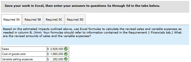
5. To evaluate alternative 2 of the proposed actions for next year, refer to the “Requirement 5 Financials” tab within your Excel workbook. Assume the company purchases new equipment in an effort to grow sales with the following estimated impacts:
- Next year’s sales and variable expenses increase by 5%.
- Next year’s fixed expenses are the same as this year.
- Next year’s ending balances in accounts receivable, inventory, and accounts payable each increase by 5% compared to their respective beginning balances.
- Next year’s ending balance in property, plant, and equipment (net) increases by $110,000 compared to its beginning balance. This reflects the purchase of a $150,000 piece of equipment minus next year’s depreciation expense of $40,000.
- Next year’s ending balance in bonds payable decreases by $50,000 compared to its beginning balance. This reflects a bond issuance of $150,000 to purchase the equipment and a bond retirement of $200,000.
- Next year’s ending balances in other assets and common stock are the same as their beginning balances.
- Based on the estimated impacts outlined above, use Excel formulas to calculate the revised sales and variable expenses as needed in column B. (Hint: Your formulas should refer to information contained in the Requirement 1 Financials tab.) What are the revised amounts of sales and the variable expenses?
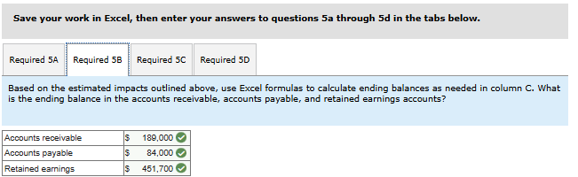
- Based on the estimated impacts outlined above, use Excel formulas to calculate ending balances as needed in column C. What is the ending balance in the accounts receivable, accounts payable, and retained earnings accounts?
- Create formulas within column D that calculate next year’s average balances for all balance sheet accounts (except Cash which will automatically be computed for you). What is the average balance in the accounts receivable, accounts payable, and retained earnings accounts?
- What is the company’s estimated average total liabilities and stockholders’ equity for next year?


15.Required information
TTo complete this activity, you will need to have Excel installed on your computer. This exercise requires you to work in Excel and answer questions in Connect. You will read a brief scenario and then download an Excel file that you will need to complete the requirements in Parts 1 through 9b of this exercise.
TSome of the requirements include brief video tutorials on using Excel functions. After viewing the tutorials, you will then use what you learned to work directly in Excel to answer the required questions in Connect.
[The following information applies to the questions displayed below.]
Edman Company is a merchandiser that has provided the following balance sheet and income statement for this year.
| Beginning Balance | Ending Balance | |
|---|---|---|
| Assets | ||
| Cash | $62,800 | $150,000 |
| Accounts receivable | 160,000 | 180,000 |
| Inventory | 230,000 | 240,000 |
| Property, plant & equipment (net) | 833,000 | 793,000 |
| Other assets | 37,000 | 37,000 |
| Total assets | $1,322,800 | $1,400,000 |
| Liabilities & Stockholders’ Equity | ||
| Accounts payable | $70,000 | $80,000 |
| Bonds payable | 550,000 | 550,000 |
| Common stock | 410,000 | 410,000 |
| Retained earnings | 292,800 | 360,000 |
| Total liabilities & stockholders’ equity | $1,322,800 | $1,400,000 |
| This Year | |
|---|---|
| Sales | $2,500,000 |
| Variable expenses: | |
| Cost of goods sold | 1,600,000 |
| Variable selling expense | 240,000 |
| Total variable expenses | 1,840,000 |
| Contribution margin | 660,000 |
| Fixed expenses: | |
| Fixed selling expenses | 220,000 |
| Fixed administrative expenses | 300,000 |
| Total fixed expenses | 520,000 |
| Net operating income | 140,000 |
| Interest expense (8%) | 44,000 |
| Net income before tax | 96,000 |
| Tax expense (30%) | 28,800 |
| Net income | $67,200 |
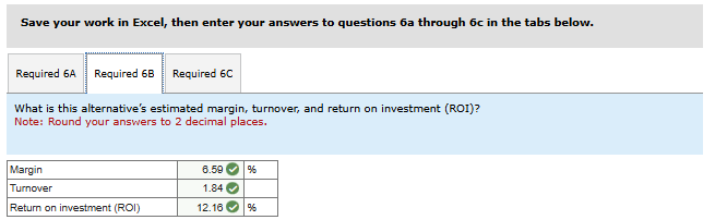
6. Refer to the “Requirement 6 DuPont Diagram” tab within your Excel workbook. For alternative 2, complete the diagram by using appropriate formulas and reference cells. (In some instances your formulas and reference cells will refer to the Requirement 5 Financials tab.)
- Which choice shows the formulas used to compute the expenses and current assets?
- What is this alternative’s estimated margin, turnover, and return on investment (ROI)?
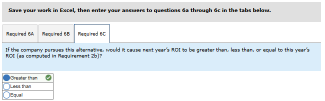
- If the company pursues this alternative, would it cause next year’s ROI to be greater than, less than, or equal to this year’s ROI (as computed in Requirement 2b)?

16.Required information
TTo complete this activity, you will need to have Excel installed on your computer. This exercise requires you to work in Excel and answer questions in Connect. You will read a brief scenario and then download an Excel file that you will need to complete the requirements in Parts 1 through 9b of this exercise.
TSome of the requirements include brief video tutorials on using Excel functions. After viewing the tutorials, you will then use what you learned to work directly in Excel to answer the required questions in Connect.
[The following information applies to the questions displayed below.]
Edman Company is a merchandiser that has provided the following balance sheet and income statement for this year.
| Beginning Balance | Ending Balance | |
|---|---|---|
| Assets | ||
| Cash | $62,800 | $150,000 |
| Accounts receivable | 160,000 | 180,000 |
| Inventory | 230,000 | 240,000 |
| Property, plant & equipment (net) | 833,000 | 793,000 |
| Other assets | 37,000 | 37,000 |
| Total assets | $1,322,800 | $1,400,000 |
| Liabilities & Stockholders’ Equity | ||
| Accounts payable | $70,000 | $80,000 |
| Bonds payable | 550,000 | 550,000 |
| Common stock | 410,000 | 410,000 |
| Retained earnings | 292,800 | 360,000 |
| Total liabilities & stockholders’ equity | $1,322,800 | $1,400,000 |
| This Year | |
|---|---|
| Sales | $2,500,000 |
| Variable expenses: | |
| Cost of goods sold | 1,600,000 |
| Variable selling expense | 240,000 |
| Total variable expenses | 1,840,000 |
| Contribution margin | 660,000 |
| Fixed expenses: | |
| Fixed selling expenses | 220,000 |
| Fixed administrative expenses | 300,000 |
| Total fixed expenses | 520,000 |
| Net operating income | 140,000 |
| Interest expense (8%) | 44,000 |
| Net income before tax | 96,000 |
| Tax expense (30%) | 28,800 |
| Net income | $67,200 |
7. To evaluate alternative 3 of the proposed actions for next year, refer to the “Requirement 7 Financials” tab within your Excel workbook. Assume the company increases its advertising expenditures (a fixed selling expense) in an effort to grow sales with the following estimated impacts:
- Next year’s sales and variable expenses increase by 30%.
- Next year’s fixed selling expense increases by $200,000.
- Next year’s ending balances in accounts receivable, inventory, and accounts payable each increase by 30% compared to their respective beginning balances.
- Next year’s ending balance in property, plant, and equipment (net) decreases by $40,000 compared to its beginning balance to reflect next year’s depreciation expense.
- Next year’s ending balances in other assets, bonds payable, and common stock are the same as their beginning balances.
- Based on the estimated impacts outlined above, use Excel formulas to calculate the revised sales, variable expenses, and fixed expenses as needed in column B. (Hint: Your formulas should refer to information contained in the “Requirement 1 Financials” tab.) What are the revised amounts of sales, the variable expenses, and the fixed selling expense?
- Based on the above estimated impacts, use Excel formulas to calculate ending balances as needed in column C. What is the ending balance in the accounts receivable, inventory, and retained earnings accounts?
- Create formulas within column D that calculate next year’s average balances for all balance sheet accounts (except Cash which will automatically be computed for you). What is the average balance in the accounts receivable, inventory, and retained earnings accounts?
- What is the company’s estimated average total liabilities and stockholders’ equity for next year?


17.Required information
TTo complete this activity, you will need to have Excel installed on your computer. This exercise requires you to work in Excel and answer questions in Connect. You will read a brief scenario and then download an Excel file that you will need to complete the requirements in Parts 1 through 9b of this exercise.
TSome of the requirements include brief video tutorials on using Excel functions. After viewing the tutorials, you will then use what you learned to work directly in Excel to answer the required questions in Connect.
[The following information applies to the questions displayed below.]
Edman Company is a merchandiser that has provided the following balance sheet and income statement for this year.
| Beginning Balance | Ending Balance | |
|---|---|---|
| Assets | ||
| Cash | $62,800 | $150,000 |
| Accounts receivable | 160,000 | 180,000 |
| Inventory | 230,000 | 240,000 |
| Property, plant & equipment (net) | 833,000 | 793,000 |
| Other assets | 37,000 | 37,000 |
| Total assets | $1,322,800 | $1,400,000 |
| Liabilities & Stockholders’ Equity | ||
| Accounts payable | $70,000 | $80,000 |
| Bonds payable | 550,000 | 550,000 |
| Common stock | 410,000 | 410,000 |
| Retained earnings | 292,800 | 360,000 |
| Total liabilities & stockholders’ equity | $1,322,800 | $1,400,000 |
| This Year | |
|---|---|
| Sales | $2,500,000 |
| Variable expenses: | |
| Cost of goods sold | 1,600,000 |
| Variable selling expense | 240,000 |
| Total variable expenses | 1,840,000 |
| Contribution margin | 660,000 |
| Fixed expenses: | |
| Fixed selling expenses | 220,000 |
| Fixed administrative expenses | 300,000 |
| Total fixed expenses | 520,000 |
| Net operating income | 140,000 |
| Interest expense (8%) | 44,000 |
| Net income before tax | 96,000 |
| Tax expense (30%) | 28,800 |
| Net income | $67,200 |
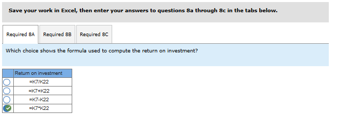
8. Refer to the “Requirement 8 DuPont Diagram” tab within your Excel workbook. For alternative 3, complete the diagram by using appropriate formulas and reference cells. (In some instances your formulas and reference cells will refer to the Requirement 7 Financials tab.)
- Which choice shows the formula used to compute the return on investment?
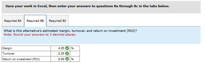
- What is this alternative’s estimated margin, turnover, and return on investment (ROI)?
- If the company pursues this alternative, would it cause next year’s ROI to be greater than, less than, or equal to this year’s ROI (as computed in Requirement 2b)?

18.Required information
To complete this activity, you will need to have Excel installed on your computer. This exercise requires you to work in Excel and answer questions in Connect. You will read a brief scenario and then download an Excel file that you will need to complete the requirements in Parts 1 through 9 of this exercise.
Some of the requirements include brief video tutorials on using Excel functions. After viewing the tutorials, you will then use what you learned to work directly in Excel to answer the required questions in Connect.
[The following information applies to the questions displayed below.]
Conroy Company manufactures two products—B100 and A200. The company provided the following information with respect to these products:
| B100 | A200 | |
|---|---|---|
| Estimated customer demand (in units) | 2,800 | 2,000 |
| Selling price per unit | $1,200 | $2,100 |
| Variable expenses per unit | $700 | $1,200 |
The company has four manufacturing departments—Fabrication, Molding, Machining, and Assemble & Pack. The capacity available in each department (in hours) and the demands that one unit of each of the company’s products makes on those departments is as follows:
| B100(hours per unit) | A200 (hours per unit) | Capacity (in hours) | |
|---|---|---|---|
| Fabrication | 1 | 2 | 4,000 |
| Molding | 2 | 2 | 6,000 |
| Machining | 2 | 0 | 5,000 |
| Assemble & Pack | 0 | 3 | 4,500 |
The company is trying to decide what product mix will maximize profits. Given that its fixed costs will not change regardless of the chosen mix, the company plans to identify the product mix that maximizes its total contribution margin.
Required:
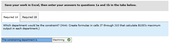
1. Refer to the “Requirements 1-3” tab in your Excel workbook. Assume the company focuses solely on producing B100:
- Create formulas in cells J7 through J10 that calculate B100’s maximum output in each department. Which department would be the constraint?
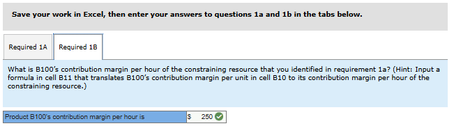
- Create a formula in cell B11 that translates B100’s contribution margin per unit in cell B10 to its contribution margin per hour of the constraining resource. What is B100’s contribution margin per hour of the constraining resource that you identified in requirement 1a?
19.Required information
To complete this activity, you will need to have Excel installed on your computer. This exercise requires you to work in Excel and answer questions in Connect. You will read a brief scenario and then download an Excel file that you will need to complete the requirements in Parts 1 through 9 of this exercise.
Some of the requirements include brief video tutorials on using Excel functions. After viewing the tutorials, you will then use what you learned to work directly in Excel to answer the required questions in Connect.
[The following information applies to the questions displayed below.]
Conroy Company manufactures two products—B100 and A200. The company provided the following information with respect to these products:
| B100 | A200 | |
|---|---|---|
| Estimated customer demand (in units) | 2,800 | 2,000 |
| Selling price per unit | $1,200 | $2,100 |
| Variable expenses per unit | $700 | $1,200 |
The company has four manufacturing departments—Fabrication, Molding, Machining, and Assemble & Pack. The capacity available in each department (in hours) and the demands that one unit of each of the company’s products makes on those departments is as follows:
| B100(hours per unit) | A200 (hours per unit) | Capacity (in hours) | |
|---|---|---|---|
| Fabrication | 1 | 2 | 4,000 |
| Molding | 2 | 2 | 6,000 |
| Machining | 2 | 0 | 5,000 |
| Assemble & Pack | 0 | 3 | 4,500 |
The company is trying to decide what product mix will maximize profits. Given that its fixed costs will not change regardless of the chosen mix, the company plans to identify the product mix that maximizes its total contribution margin.
2. Refer to the “Requirements 1-3” tab in your Excel workbook. Assume the company focuses solely on producing A200:
- Which department would be its constraint? (Hint: Create formulas in cells K7 through K10 that calculate A200’s maximum output in each department.)
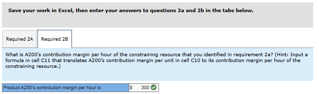
- What is A200’s contribution margin per hour of the constraining resource that you identified in requirement 2a? (Hint: Input a formula in cell C11 that translates A200’s contribution margin per unit in cell C10 to its contribution margin per hour of the constraining resource.)

20.Required information
To complete this activity, you will need to have Excel installed on your computer. This exercise requires you to work in Excel and answer questions in Connect. You will read a brief scenario and then download an Excel file that you will need to complete the requirements in Parts 1 through 9 of this exercise.
Some of the requirements include brief video tutorials on using Excel functions. After viewing the tutorials, you will then use what you learned to work directly in Excel to answer the required questions in Connect.
[The following information applies to the questions displayed below.]
Conroy Company manufactures two products—B100 and A200. The company provided the following information with respect to these products:
| B100 | A200 | |
|---|---|---|
| Estimated customer demand (in units) | 2,800 | 2,000 |
| Selling price per unit | $1,200 | $2,100 |
| Variable expenses per unit | $700 | $1,200 |
The company has four manufacturing departments—Fabrication, Molding, Machining, and Assemble & Pack. The capacity available in each department (in hours) and the demands that one unit of each of the company’s products makes on those departments is as follows:
| B100(hours per unit) | A200 (hours per unit) | Capacity (in hours) | |
|---|---|---|---|
| Fabrication | 1 | 2 | 4,000 |
| Molding | 2 | 2 | 6,000 |
| Machining | 2 | 0 | 5,000 |
| Assemble & Pack | 0 | 3 | 4,500 |
The company is trying to decide what product mix will maximize profits. Given that its fixed costs will not change regardless of the chosen mix, the company plans to identify the product mix that maximizes its total contribution margin.
3. Refer to the “Requirements 1-3” tab in your Excel workbook. Based on the answers to requirements 1 and 2:
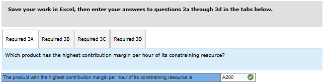
- Which product has the highest contribution margin per hour of its constraining resource?
- If the company decided to initiate production by maximizing the output of the product chosen in requirement 3a, then how many units of this product would it be able to make before encountering that product’s constraint?
- Input your answer from requirement 3b into the appropriate cell, either cell B7 or C7. Then, direct your attention to the unused capacities in cells J15 through J18. If the company implemented the production plan in requirement 3b, then how many units of its remaining product could it make with the capacity that is still available?
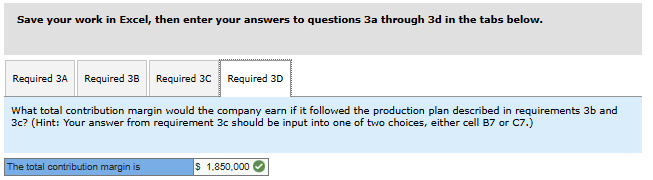
- What total contribution margin would the company earn if it followed the production plan described in requirements 3b and 3c? Input your answer from requirement 3c into the appropriate cell, either cell B7 or C7. What total contribution margin would the company earn if it followed the production plan described in requirements 3b and 3c?


21.Required information
To complete this activity, you will need to have Excel installed on your computer. This exercise requires you to work in Excel and answer questions in Connect. You will read a brief scenario and then download an Excel file that you will need to complete the requirements in Parts 1 through 9 of this exercise.
Some of the requirements include brief video tutorials on using Excel functions. After viewing the tutorials, you will then use what you learned to work directly in Excel to answer the required questions in Connect.
[The following information applies to the questions displayed below.]
Conroy Company manufactures two products—B100 and A200. The company provided the following information with respect to these products:
| B100 | A200 | |
|---|---|---|
| Estimated customer demand (in units) | 2,800 | 2,000 |
| Selling price per unit | $1,200 | $2,100 |
| Variable expenses per unit | $700 | $1,200 |
The company has four manufacturing departments—Fabrication, Molding, Machining, and Assemble & Pack. The capacity available in each department (in hours) and the demands that one unit of each of the company’s products makes on those departments is as follows:
| B100(hours per unit) | A200 (hours per unit) | Capacity (in hours) | |
|---|---|---|---|
| Fabrication | 1 | 2 | 4,000 |
| Molding | 2 | 2 | 6,000 |
| Machining | 2 | 0 | 5,000 |
| Assemble & Pack | 0 | 3 | 4,500 |
The company is trying to decide what product mix will maximize profits. Given that its fixed costs will not change regardless of the chosen mix, the company plans to identify the product mix that maximizes its total contribution margin.
Click here for a brief tutorial on SOLVER in Excel.
4. In the Excel workbook, navigate to the “Requirement 4” tab. Using Solver:
- Calculate the maximum contribution margin the company can earn given the capacities of its four manufacturing departments.
- How many units of each product would the company produce to earn the contribution margin from requirement 4a?
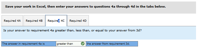
- Is your answer to requirement 4a greater than, less than, or equal to your answer from 3d?
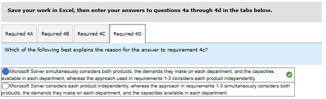
- Which of the following best explains the reason for the answer to requirement 4c?


22.Required information
To complete this activity, you will need to have Excel installed on your computer. This exercise requires you to work in Excel and answer questions in Connect. You will read a brief scenario and then download an Excel file that you will need to complete the requirements in Parts 1 through 9 of this exercise.
Some of the requirements include brief video tutorials on using Excel functions. After viewing the tutorials, you will then use what you learned to work directly in Excel to answer the required questions in Connect.
[The following information applies to the questions displayed below.]
Conroy Company manufactures two products—B100 and A200. The company provided the following information with respect to these products:
| B100 | A200 | |
|---|---|---|
| Estimated customer demand (in units) | 2,800 | 2,000 |
| Selling price per unit | $1,200 | $2,100 |
| Variable expenses per unit | $700 | $1,200 |
The company has four manufacturing departments—Fabrication, Molding, Machining, and Assemble & Pack. The capacity available in each department (in hours) and the demands that one unit of each of the company’s products makes on those departments is as follows:
| B100(hours per unit) | A200 (hours per unit) | Capacity (in hours) | |
|---|---|---|---|
| Fabrication | 1 | 2 | 4,000 |
| Molding | 2 | 2 | 6,000 |
| Machining | 2 | 0 | 5,000 |
| Assemble & Pack | 0 | 3 | 4,500 |
The company is trying to decide what product mix will maximize profits. Given that its fixed costs will not change regardless of the chosen mix, the company plans to identify the product mix that maximizes its total contribution margin.
Click here for a a brief tutorial on Charts in Excel.
5. In the Excel workbook, navigate to the “Requirement 5” tab. Using Charts, prepare a graph using the following three guidelines:
- First, label the X-axis B100: Units Produced and the Y-axis A200: Units Produced. Then establish a range on each axis of 0 – 4,000 units.
- Second, plot four lines that depict the production possibilities within each of the four departments. For example, the Fabrication Department could produce a maximum of 4,000 units of B100 (= 4,000 hours available ÷ 1 hour per unit) or a maximum of 2,000 units of A200 (= 4,000 hours available ÷ 2 hours per unit). Thus, this line should connect two data points, 4,000 units on the X-axis and 2,000 units on the Y-axis.
- Third, once you have plotted all four lines, pay particular attention to the portion of the graph that is enclosed by the four lines because it depicts the full range of Conroy’s production possibilities.
1.Based on the graph you created, which of the statements below are true?
Note: You may select more than one answer. Single click the box with the question mark to produce a check mark for a correct answer or double click the box with the question mark to empty the box for a wrong answer. Any boxes left with a question mark will be automatically graded as incorrect.

23.Required information
To complete this activity, you will need to have Excel installed on your computer. This exercise requires you to work in Excel and answer questions in Connect. You will read a brief scenario and then download an Excel file that you will need to complete the requirements in Parts 1 through 9 of this exercise.
Some of the requirements include brief video tutorials on using Excel functions. After viewing the tutorials, you will then use what you learned to work directly in Excel to answer the required questions in Connect.
[The following information applies to the questions displayed below.]
Conroy Company manufactures two products—B100 and A200. The company provided the following information with respect to these products:
| B100 | A200 | |
|---|---|---|
| Estimated customer demand (in units) | 2,800 | 2,000 |
| Selling price per unit | $1,200 | $2,100 |
| Variable expenses per unit | $700 | $1,200 |
The company has four manufacturing departments—Fabrication, Molding, Machining, and Assemble & Pack. The capacity available in each department (in hours) and the demands that one unit of each of the company’s products makes on those departments is as follows:
| B100(hours per unit) | A200 (hours per unit) | Capacity (in hours) | |
|---|---|---|---|
| Fabrication | 1 | 2 | 4,000 |
| Molding | 2 | 2 | 6,000 |
| Machining | 2 | 0 | 5,000 |
| Assemble & Pack | 0 | 3 | 4,500 |
The company is trying to decide what product mix will maximize profits. Given that its fixed costs will not change regardless of the chosen mix, the company plans to identify the product mix that maximizes its total contribution margin.
6. In the Excel workbook, refer to the graph you prepared for requirement 5 to answer the following questions:
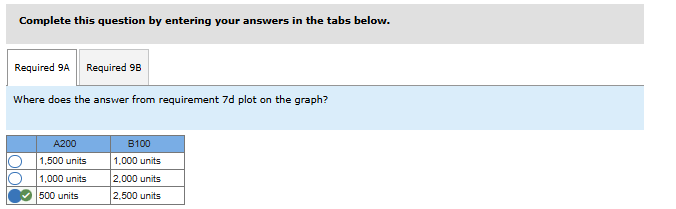
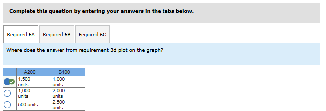
- Consider your answer from requirement 3d. At which point would it plot on the graph?
- Consider your answer from requirement 4a. At which point would it plot on the graph?
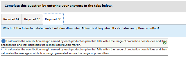
- Which of the following statements best describes what Solver is doing when it calculates an optimal solution?

24.Required information
To complete this activity, you will need to have Excel installed on your computer. This exercise requires you to work in Excel and answer questions in Connect. You will read a brief scenario and then download an Excel file that you will need to complete the requirements in Parts 1 through 9 of this exercise.
Some of the requirements include brief video tutorials on using Excel functions. After viewing the tutorials, you will then use what you learned to work directly in Excel to answer the required questions in Connect.
[The following information applies to the questions displayed below.]
Conroy Company manufactures two products—B100 and A200. The company provided the following information with respect to these products:
| B100 | A200 | |
|---|---|---|
| Estimated customer demand (in units) | 2,800 | 2,000 |
| Selling price per unit | $1,200 | $2,100 |
| Variable expenses per unit | $700 | $1,200 |
The company has four manufacturing departments—Fabrication, Molding, Machining, and Assemble & Pack. The capacity available in each department (in hours) and the demands that one unit of each of the company’s products makes on those departments is as follows:
| B100(hours per unit) | A200 (hours per unit) | Capacity (in hours) | |
|---|---|---|---|
| Fabrication | 1 | 2 | 4,000 |
| Molding | 2 | 2 | 6,000 |
| Machining | 2 | 0 | 5,000 |
| Assemble & Pack | 0 | 3 | 4,500 |
The company is trying to decide what product mix will maximize profits. Given that its fixed costs will not change regardless of the chosen mix, the company plans to identify the product mix that maximizes its total contribution margin.
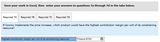
7. In the Excel workbook, navigate to the “Requirement 7” tab. Assume that Conroy is considering raising the price of B100 to $1,400. The company believes that the price increase would drop maximum customer demand from 2,800 units to 2,600 units. Input the appropriate values and create formulas as necessary on the Excel worksheet to answer the following questions:
- If Conroy implements the price increase, which product would have the highest contribution margin per unit of its constraining resource?
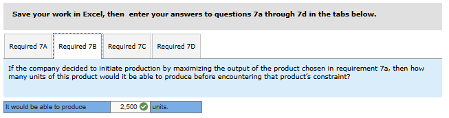
- If the company decided to initiate production by maximizing the output of the product chosen in requirement 7a, then how many units of this product would it be able to produce before encountering that product’s constraint?
- If the company implemented the production plan in requirement 7b, then how many units of its remaining product could it produce with the capacity that is still available?
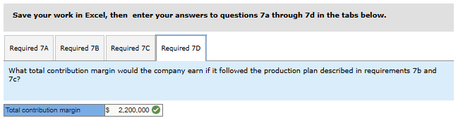
- What total contribution margin would the company earn if it followed the production plan described in requirements 7b and 7c?

25.Required information
To complete this activity, you will need to have Excel installed on your computer. This exercise requires you to work in Excel and answer questions in Connect. You will read a brief scenario and then download an Excel file that you will need to complete the requirements in Parts 1 through 9 of this exercise.
Some of the requirements include brief video tutorials on using Excel functions. After viewing the tutorials, you will then use what you learned to work directly in Excel to answer the required questions in Connect.
[The following information applies to the questions displayed below.]
Conroy Company manufactures two products—B100 and A200. The company provided the following information with respect to these products:
| B100 | A200 | |
|---|---|---|
| Estimated customer demand (in units) | 2,800 | 2,000 |
| Selling price per unit | $1,200 | $2,100 |
| Variable expenses per unit | $700 | $1,200 |
The company has four manufacturing departments—Fabrication, Molding, Machining, and Assemble & Pack. The capacity available in each department (in hours) and the demands that one unit of each of the company’s products makes on those departments is as follows:
| B100(hours per unit) | A200 (hours per unit) | Capacity (in hours) | |
|---|---|---|---|
| Fabrication | 1 | 2 | 4,000 |
| Molding | 2 | 2 | 6,000 |
| Machining | 2 | 0 | 5,000 |
| Assemble & Pack | 0 | 3 | 4,500 |
The company is trying to decide what product mix will maximize profits. Given that its fixed costs will not change regardless of the chosen mix, the company plans to identify the product mix that maximizes its total contribution margin.
8. In the Excel workbook, navigate to the “Requirement 8” tab. Use Excel’s Solver function to answer the following:
- What is the maximum contribution margin the company can earn with its available resources if it increases the price of B100 to $1,400?
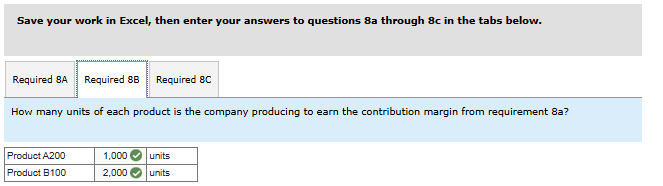
- How many units of each product is the company producing to earn the contribution margin from requirement 8a?
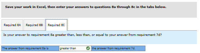
- Is your answer to requirement 8a greater than, less than, or equal to your answer from requirement 7d?

26.Required information
To complete this activity, you will need to have Excel installed on your computer. This exercise requires you to work in Excel and answer questions in Connect. You will read a brief scenario and then download an Excel file that you will need to complete the requirements in Parts 1 through 9 of this exercise.
Some of the requirements include brief video tutorials on using Excel functions. After viewing the tutorials, you will then use what you learned to work directly in Excel to answer the required questions in Connect.
[The following information applies to the questions displayed below.]
Conroy Company manufactures two products—B100 and A200. The company provided the following information with respect to these products:
| B100 | A200 | |
|---|---|---|
| Estimated customer demand (in units) | 2,800 | 2,000 |
| Selling price per unit | $1,200 | $2,100 |
| Variable expenses per unit | $700 | $1,200 |
The company has four manufacturing departments—Fabrication, Molding, Machining, and Assemble & Pack. The capacity available in each department (in hours) and the demands that one unit of each of the company’s products makes on those departments is as follows:
| B100(hours per unit) | A200 (hours per unit) | Capacity (in hours) | |
|---|---|---|---|
| Fabrication | 1 | 2 | 4,000 |
| Molding | 2 | 2 | 6,000 |
| Machining | 2 | 0 | 5,000 |
| Assemble & Pack | 0 | 3 | 4,500 |
The company is trying to decide what product mix will maximize profits. Given that its fixed costs will not change regardless of the chosen mix, the company plans to identify the product mix that maximizes its total contribution margin.
9. In the Excel workbook, refer to the graph you prepared for requirement 5 to answer the following questions:
- Consider your answer from requirement 7d. At which point would it plot on the graph?
- Consider your answer from requirement 8a. At which point would it plot on the graph?