
1) Binary classification
There are two types of supervised learning—classification and regression. Binary classification is used to predict a target variable that has only two labels, typically represented numerically with a zero or a one.
The .head() of a dataset, churn_df, is shown below. You can expect the rest of the data to contain similar values.
account_length total_day_charge total_eve_charge total_night_charge total_intl_charge customer_service_calls churn
0 101 45.85 17.65 9.64 1.22 3 1
1 73 22.30 9.05 9.98 2.75 2 0
2 86 24.62 17.53 11.49 3.13 4 0
3 59 34.73 21.02 9.66 3.24 1 0
4 129 27.42 18.75 10.11 2.59 1 0
Looking at this data, which column could be the target variable for binary classification?

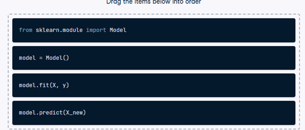
2) The supervised learning workflow
Recall that scikit-learn offers a repeatable workflow for using supervised learning models to predict the target variable values when presented with new data.
Reorder the pseudo-code provided so it accurately represents the workflow of building a supervised learning model and making predictions.
- Drag the code blocks into the correct order to represent how a supervised learning workflow would be executed.
3) k-Nearest Neighbors: Fit
In this exercise, you will build your first classification model using the churn_df dataset, which has been preloaded for the remainder of the chapter.
The target, “churn”, needs to be a single column with the same number of observations as the feature data. The feature data has already been converted into numpy arrays.
“account_length” and “customer_service_calls” are treated as features because account length indicates customer loyalty, and frequent customer service calls may signal dissatisfaction, both of which can be good predictors of churn.
- Import KNeighborsClassifier from sklearn.neighbors.
- Instantiate a KNeighborsClassifier called knn with 6 neighbors.
- Fit the classifier to the data using the .fit() method.
# Import KNeighborsClassifier
from sklearn.neighbors import KNeighborsClassifier
y = churn_df[“churn”].values
X = churn_df[[“account_length”, “customer_service_calls”]].values
# Create a KNN classifier with 6 neighbors
knn = KNeighborsClassifier(n_neighbors=6)
# Fit the classifier to the data
knn.fit(X, y)
4) k-Nearest Neighbors: Predict
Now you have fit a KNN classifier, you can use it to predict the label of new data points. All available data was used for training, however, fortunately, there are new observations available. These have been preloaded for you as X_new.
The model knn, which you created and fit the data in the last exercise, has been preloaded for you. You will use your classifier to predict the labels of a set of new data points:
X_new = np.array([[30.0, 17.5],
[107.0, 24.1],
[213.0, 10.9]])
- Create y_pred by predicting the target values of the unseen features X_new using the knn model.
- Print the predicted labels for the set of predictions.
# Predict the labels for the X_new
y_pred = knn.predict(X_new)
# Print the predictions
print(“Predictions: {}”.format(y_pred))
5) Train/test split + computing accuracy
It’s time to practice splitting your data into training and test sets with the churn_df dataset!
NumPy arrays have been created for you containing the features as X and the target variable as y.
- Import train_test_split from sklearn.model_selection.
- Split X and y into training and test sets, setting test_size equal to 20%, random_state to 42, and ensuring the target label proportions reflect that of the original dataset.
- Fit the knn model to the training data.
- Compute and print the model’s accuracy for the test data.
# Import the module
from sklearn.model_selection import train_test_split
X = churn_df.drop(“churn”, axis=1).values
y = churn_df[“churn”].values
# Split into training and test sets
X_train, X_test, y_train, y_test = train_test_split(
X, y, test_size=0.2, random_state=42, stratify=y
)
knn = KNeighborsClassifier(n_neighbors=5)
# Fit the classifier to the training data
knn.fit(X_train, y_train)
# Print the accuracy
print(knn.score(X_test, y_test))
6) Overfitting and underfitting
Interpreting model complexity is a great way to evaluate supervised learning performance. Your aim is to produce a model that can interpret the relationship between features and the target variable, as well as generalize well when exposed to new observations.
The training and test sets have been created from the churn_df dataset and preloaded as X_train, X_test, y_train, and y_test.
In addition, KNeighborsClassifier has been imported for you along with numpy as np.
- Create neighbors as a numpy array of values from 1 up to and including 12.
- Instantiate a KNeighborsClassifier, with the number of neighbors equal to the neighbor iterator.
- Fit the model to the training data.
- Calculate accuracy scores for the training set and test set separately using the .score() method, and assign the results to the train_accuracies and test_accuracies dictionaries, respectively, utilizing the neighbor iterator as the index.
# Create neighbors
neighbors = np.arange(1, 13)
train_accuracies = {}
test_accuracies = {}
for neighbor in neighbors:
# Set up a KNN Classifier
knn = KNeighborsClassifier(n_neighbors=neighbor)
# Fit the model
knn.fit(X_train, y_train)
# Compute accuracy
train_accuracies[neighbor] = knn.score(X_train, y_train)
test_accuracies[neighbor] = knn.score(X_test, y_test)
print(neighbors, ‘\n’, train_accuracies, ‘\n’, test_accuracies)
7) Visualizing model complexity
Now you have calculated the accuracy of the KNN model on the training and test sets using various values of n_neighbors, you can create a model complexity curve to visualize how performance changes as the model becomes less complex!
The variables neighbors, train_accuracies, and test_accuracies, which you generated in the previous exercise, have all been preloaded for you. You will plot the results to aid in finding the optimal number of neighbors for your model.
- Add a title “KNN: Varying Number of Neighbors”.
- Plot the .values() method of train_accuracies on the y-axis against neighbors on the x-axis, with a label of “Training Accuracy”.
- Plot the .values() method of test_accuracies on the y-axis against neighbors on the x-axis, with a label of “Testing Accuracy”.
- Display the plot.
# Add a title
plt.title(“KNN: Varying Number of Neighbors”)
# Plot training accuracies
plt.plot(neighbors, train_accuracies.values(), label=”Training Accuracy”)
# Plot test accuracies
plt.plot(neighbors, test_accuracies.values(), label=”Testing Accuracy”)
plt.legend()
plt.xlabel(“Number of Neighbors”)
plt.ylabel(“Accuracy”)
# Display the plot
plt.show()
8) Creating features
In this chapter, you will work with a dataset called sales_df, which contains information on advertising campaign expenditure across different media types, and the number of dollars generated in sales for the respective campaign. The dataset has been preloaded for you. Here are the first two rows:
tv radio social_media sales
1 13000.0 9237.76 2409.57 46677.90
2 41000.0 15886.45 2913.41 150177.83
You will use the advertising expenditure as features to predict sales values, initially working with the “radio” column. However, before you make any predictions you will need to create the feature and target arrays, reshaping them to the correct format for scikit-learn.
- Create X, an array of the values from the sales_df DataFrame’s “radio” column.
- Create y, an array of the values from the sales_df DataFrame’s “sales” column.
- Reshape X into a two-dimensional NumPy array.
- Print the shape of X and y.
import numpy as np
# Create X from the radio column’s values
X = sales_df[“radio”].values
# Create y from the sales column’s values
y = sales_df[“sales”].values
# Reshape X
X = X.reshape(-1, 1)
# Check the shape of the features and targets
print(X.shape, y.shape)
9) Building a linear regression model
Now you have created your feature and target arrays, you will train a linear regression model on all feature and target values.
As the goal is to assess the relationship between the feature and target values there is no need to split the data into training and test sets.
X and y have been preloaded for you as follows:
y = sales_df[“sales”].values
X = sales_df[“radio”].values.reshape(-1, 1)
- Import LinearRegression.
- Instantiate a linear regression model.
- Predict sales values using X, storing as predictions.
# Import LinearRegression
from sklearn.linear_model import LinearRegression
# Create the model
reg = LinearRegression()
# Fit the model to the data
reg.fit(X, y)
# Make predictions
predictions = reg.predict(X)
print(predictions[:5])
10) Visualizing a linear regression model
Now you have built your linear regression model and trained it using all available observations, you can visualize how well the model fits the data. This allows you to interpret the relationship between radio advertising expenditure and sales values.
The variables X, an array of radio values, y, an array of sales values, and predictions, an array of the model’s predicted values for y given X, have all been preloaded for you from the previous exercise.
- Import matplotlib.pyplot as plt.
- Create a scatter plot visualizing y against X, with observations in blue.
- Draw a red line plot displaying the predictions against X.
- Display the plot.
# Import matplotlib.pyplot
import matplotlib.pyplot as plt
# Create scatter plot
plt.scatter(X, y, color=”blue”)
# Create line plot
plt.plot(X, predictions, color=”red”)
plt.xlabel(“Radio Expenditure ($)”)
plt.ylabel(“Sales ($)”)
# Display the plot
plt.show()
11) Fit and predict for regression
Now you have seen how linear regression works, your task is to create a multiple linear regression model using all of the features in the sales_df dataset, which has been preloaded for you. As a reminder, here are the first two rows:
tv radio social_media sales
1 13000.0 9237.76 2409.57 46677.90
2 41000.0 15886.45 2913.41 150177.83
You will then use this model to predict sales based on the values of the test features.
LinearRegression and train_test_split have been preloaded for you from their respective modules.
- Create X, an array containing values of all features in sales_df, and y, containing all values from the “sales” column.
- Instantiate a linear regression model.
- Fit the model to the training data.
- Create y_pred, making predictions for sales using the test features.
# Create X and y arrays
X = sales_df.drop(“sales”, axis=1).values
y = sales_df[“sales”].values
X_train, X_test, y_train, y_test = train_test_split(X, y, test_size=0.3, random_state=42)
# Instantiate the model
reg = LinearRegression()
# Fit the model to the data
reg.fit(X_train, y_train)
# Make predictions
y_pred = reg.predict(X_test)
print(“Predictions: {}, Actual Values: {}”.format(y_pred[:2], y_test[:2]))
12) Regression performance
Now you have fit a model, reg, using all features from sales_df, and made predictions of sales values, you can evaluate performance using some common regression metrics.
The variables X_train, X_test, y_train, y_test, and y_pred, along with the fitted model, reg, all from the last exercise, have been preloaded for you.
Your task is to find out how well the features can explain the variance in the target values, along with assessing the model’s ability to make predictions on unseen data.
- Import root_mean_squared_error.
- Calculate the model’s R-squared score by passing the test feature values and the test target values to an appropriate method.
- Calculate the model’s root mean squared error using y_test and y_pred.
- Print r_squared and rmse.
# Import root_mean_squared_error
from sklearn.metrics import root_mean_squared_error
# Compute R-squared
r_squared = reg.score(X_test, y_test)
# Compute RMSE
rmse = root_mean_squared_error(y_test, y_pred)
# Print the metrics
print(“R^2: {}”.format(r_squared))
print(“RMSE: {}”.format(rmse))
13) Cross-validation for R-squared
Cross-validation is a vital approach to evaluating a model. It maximizes the amount of data that is available to the model, as the model is not only trained but also tested on all of the available data.
In this exercise, you will build a linear regression model, then use 6-fold cross-validation to assess its accuracy for predicting sales using social media advertising expenditure. You will display the individual score for each of the six-folds.
The sales_df dataset has been split into y for the target variable, and X for the features, and preloaded for you. LinearRegression has been imported from sklearn.linear_model.
- Import KFold and cross_val_score.
- Create kf by calling KFold(), setting the number of splits to six, shuffle to True, and setting a seed of 5.
- Perform cross-validation using reg on X and y, passing kf to cv.
- Print the cv_scores.
# Import the necessary modules
from sklearn.model_selection import KFold, cross_val_score
# Create a KFold object
kf = KFold(n_splits=6, shuffle=True, random_state=5)
reg = LinearRegression()
# Compute 6-fold cross-validation scores
cv_scores = cross_val_score(reg, X, y, cv=kf)
# Print scores
print(cv_scores)
14) Analyzing cross-validation metrics
Now you have performed cross-validation, it’s time to analyze the results.
You will display the mean, standard deviation, and 95% confidence interval for cv_results, which has been preloaded for you from the previous exercise.
numpy has been imported for you as np.
- Calculate and print the mean of the results.
- Calculate and print the standard deviation of cv_results.
- Display the 95% confidence interval for your results using np.quantile().
# Print the mean
print(np.mean(cv_results))
# Print the standard deviation
print(np.std(cv_results))
# Print the 95% confidence interval
print(np.quantile(cv_results, [0.025, 0.975]))
15) Regularized regression: Ridge
Ridge regression performs regularization by computing the squared values of the model parameters multiplied by alpha and adding them to the loss function.
In this exercise, you will fit ridge regression models over a range of different alpha values, and print their scores. You will use all of the features in the sales_df dataset to predict “sales”. The data has been split into X_train, X_test, y_train, y_test for you.
A variable called alphas has been provided as a list containing different alpha values, which you will loop through to generate scores.
- Import Ridge.
- Instantiate Ridge, setting alpha equal to alpha.
- Fit the model to the training data.
- Calculate the
score for each iteration of ridge.
# Import Ridge
from sklearn.linear_model import Ridge
alphas = [0.1, 1.0, 10.0, 100.0, 1000.0, 10000.0]
ridge_scores = []
for alpha in alphas:
# Create a Ridge regression model
ridge = Ridge(alpha=alpha)
# Fit the data
ridge.fit(X_train, y_train)
# Obtain R-squared
score = ridge.score(X_test, y_test)
ridge_scores.append(score)
print(ridge_scores)
16) Lasso regression for feature importance
In the video, you saw how lasso regression can be used to identify important features in a dataset.
In this exercise, you will fit a lasso regression model to the sales_df data and plot the model’s coefficients.
The feature and target variable arrays have been pre-loaded as X and y, along with sales_columns, which contains the dataset’s feature names.
- Import Lasso from sklearn.linear_model.
- Instantiate a Lasso regressor with an alpha of 0.3.
- Fit the model to the data.
- Compute the model’s coefficients, storing as lasso_coef.
# Import Lasso
from sklearn.linear_model import Lasso
# Instantiate a lasso regression model
lasso = Lasso(alpha=0.3)
# Fit the model to the data
lasso.fit(X, y)
# Compute and print the coefficients
lasso_coef = lasso.coef_
print(lasso_coef)
plt.bar(sales_columns, lasso_coef)
plt.xticks(rotation=45)
plt.show()
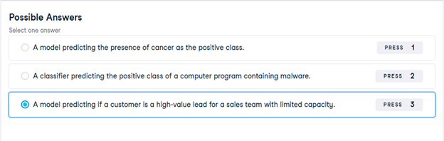
17) Deciding on a primary metric
As you have seen, several metrics can be useful to evaluate the performance of classification models, including accuracy, precision, recall, and F1-score.
In this exercise, you will be provided with three different classification problems, and your task is to select the problem where precision is best suited as the primary metric.
18) Assessing a diabetes prediction classifier
In this chapter you’ll work with the diabetes_df dataset introduced previously.
The goal is to predict whether or not each individual is likely to have diabetes based on the features body mass index (BMI) and age (in years). Therefore, it is a binary classification problem. A target value of 0 indicates that the individual does not have diabetes, while a value of 1 indicates that the individual does have diabetes.
diabetes_df has been preloaded for you as a pandas DataFrame and split into X_train, X_test, y_train, and y_test. In addition, a KNeighborsClassifier() has been instantiated and assigned to knn.
You will fit the model, make predictions on the test set, then produce a confusion matrix and classification report.
- Import confusion_matrix and classification_report.
- Fit the model to the training data.
- Predict the labels of the test set, storing the results as y_pred.
- Compute and print the confusion matrix and classification report for the test labels versus the predicted labels.
# Import confusion matrix and classification report
from sklearn.metrics import confusion_matrix, classification_report
knn = KNeighborsClassifier(n_neighbors=6)
# Fit the model to the training data
knn.fit(X_train, y_train)
# Predict the labels of the test data: y_pred
y_pred = knn.predict(X_test)
# Generate the confusion matrix and classification report
print(confusion_matrix(y_test, y_pred))
print(classification_report(y_test, y_pred))
19) Building a logistic regression model
In this exercise, you will build a logistic regression model using all features in the diabetes_df dataset. The model will be used to predict the probability of individuals in the test set having a diabetes diagnosis.
The diabetes_df dataset has been split into X_train, X_test, y_train, and y_test, and preloaded for you.
- Import LogisticRegression.
- Instantiate a logistic regression model, logreg.
- Fit the model to the training data.
- Predict the probabilities of each individual in the test set having a diabetes diagnosis, storing the array of positive probabilities as y_pred_probs.
# Import LogisticRegression
from sklearn.linear_model import LogisticRegression
# Instantiate the model
logreg = LogisticRegression()
# Fit the model
logreg.fit(X_train, y_train)
# Predict probabilities
y_pred_probs = logreg.predict_proba(X_test)[:, 1]
print(y_pred_probs[:10])
20) The ROC curve
Now you have built a logistic regression model for predicting diabetes status, you can plot the ROC curve to visualize how the true positive rate and false positive rate vary as the decision threshold changes.
The test labels, y_test, and the predicted probabilities of the test features belonging to the positive class, y_pred_probs, have been preloaded for you, along with matplotlib.pyplot as plt.
You will create a ROC curve and then interpret the results.
- Import roc_curve.
- Calculate the ROC curve values, using y_test and y_pred_probs, and unpacking the results into fpr, tpr, and thresholds.
- Plot true positive rate against false positive rate.
# Import roc_curve
from sklearn.metrics import roc_curve
# Generate ROC curve values: fpr, tpr, thresholds
fpr, tpr, thresholds = roc_curve(y_test, y_pred_probs)
plt.plot([0, 1], [0, 1], ‘k–‘)
# Plot tpr against fpr
plt.plot(fpr, tpr)
plt.xlabel(‘False Positive Rate’)
plt.ylabel(‘True Positive Rate’)
plt.title(‘ROC Curve for Diabetes Prediction’)
plt.show()
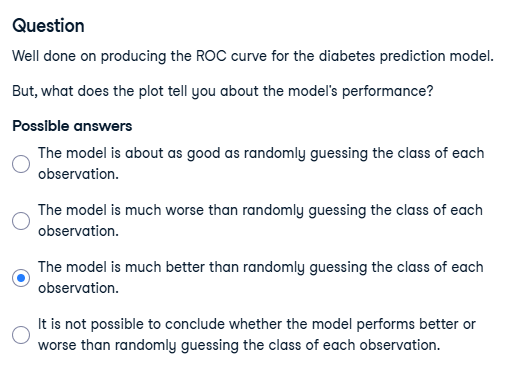
21) ROC AUC
The ROC curve you plotted in the last exercise looked promising.
Now you will compute the area under the ROC curve, along with the other classification metrics you have used previously.
The confusion_matrix and classification_report functions have been preloaded for you, along with the logreg model you previously built, plus X_train, X_test, y_train, y_test. Also, the model’s predicted test set labels are stored as y_pred, and probabilities of test set observations belonging to the positive class stored as y_pred_probs.
A knn model has also been created and the performance metrics printed in the console, so you can compare the roc_auc_score, confusion_matrix, and classification_report between the two models.
- Import roc_auc_score.
- Calculate and print the ROC AUC score, passing the test labels and the predicted positive class probabilities.
- Calculate and print the confusion matrix.
- Call classification_report().
# Import roc_auc_score
from sklearn.metrics import roc_auc_score
# Calculate roc_auc_score
print(roc_auc_score(y_test, y_pred_probs))
# Calculate the confusion matrix
print(confusion_matrix(y_test, y_pred))
# Calculate the classification report
print(classification_report(y_test, y_pred))
22) Hyperparameter tuning with GridSearchCV
Now you have seen how to perform grid search hyperparameter tuning, you are going to build a lasso regression model with optimal hyperparameters to predict blood glucose levels using the features in the diabetes_df dataset.
X_train, X_test, y_train, and y_test have been preloaded for you. A KFold() object has been created and stored for you as kf, along with a lasso regression model as lasso.
- Import GridSearchCV.
- Set up a parameter grid for “alpha”, using np.linspace() to create 20 evenly spaced values ranging from 0.00001 to 1.
- Call GridSearchCV(), passing lasso, the parameter grid, and setting cv equal to kf.
- Fit the grid search object to the training data to perform a cross-validated grid search.
# Import GridSearchCV
from sklearn.model_selection import GridSearchCV
# Set up the parameter grid
param_grid = {“alpha”: np.linspace(0.00001, 1, 20)}
# Instantiate lasso_cv
lasso_cv = GridSearchCV(lasso, param_grid, cv=kf)
# Fit to the training data
lasso_cv.fit(X_train, y_train)
print(“Tuned lasso paramaters: {}”.format(lasso_cv.best_params_))
print(“Tuned lasso score: {}”.format(lasso_cv.best_score_))
23) Hyperparameter tuning with RandomizedSearchCV
As you saw, GridSearchCV can be computationally expensive, especially if you are searching over a large hyperparameter space. In this case, you can use RandomizedSearchCV, which tests a fixed number of hyperparameter settings from specified probability distributions.
Training and test sets from diabetes_df have been pre-loaded for you as X_train. X_test, y_train, and y_test, where the target is “diabetes”. A logistic regression model has been created and stored as logreg, as well as a KFold variable stored as kf.
You will define a range of hyperparameters and use RandomizedSearchCV, which has been imported from sklearn.model_selection, to look for optimal hyperparameters from these options.
- Create params, adding “l1” and “l2” as penalty values, setting C to a range of 50 float values between 0.1 and 1.0, and class_weight to either “balanced” or a dictionary containing 0:0.8, 1:0.2.
- Create the Randomized Search CV object, passing the model and the parameters, and setting cv equal to kf.
- Fit logreg_cv to the training data.
- Print the model’s best parameters and accuracy score.
# Create the parameter space
params = {“penalty”: [“l1”, “l2”],
“tol”: np.linspace(0.0001, 1.0, 50),
“C”: np.linspace(0.1, 1.0, 50),
“class_weight”: [“balanced”, {0: 0.8, 1: 0.2}]}
# Instantiate the RandomizedSearchCV object
logreg_cv = RandomizedSearchCV(logreg, params, cv=kf)
# Fit the data to the model
logreg_cv.fit(X_train, y_train)
# Print the tuned parameters and score
print(“Tuned Logistic Regression Parameters: {}”.format(logreg_cv.best_params_))
print(“Tuned Logistic Regression Best Accuracy Score: {}”.format(logreg_cv.best_score_))
24) Creating dummy variables
Being able to include categorical features in the model building process can enhance performance as they may add information that contributes to prediction accuracy.
The music_df dataset has been preloaded for you, and its shape is printed. Also, pandas has been imported as pd.
Now you will create a new DataFrame containing the original columns of music_df plus dummy variables from the “genre” column.
- Use a relevant function, passing the entire music_df DataFrame, to create music_dummies, dropping the first binary column.
- Print the shape of music_dummies.
# Create music_dummies
music_dummies = pd.get_dummies(music_df, drop_first=True)
# Print the new DataFrame’s shape
print(“Shape of music_dummies: {}”.format(music_dummies.shape))
25) Regression with categorical features
Now you have created music_dummies, containing binary features for each song’s genre, it’s time to build a ridge regression model to predict song popularity.
music_dummies has been preloaded for you, along with Ridge, cross_val_score, numpy as np, and a KFold object stored as kf.
The model will be evaluated by calculating the average RMSE, but first, you will need to convert the scores for each fold to positive values and take their square root. This metric shows the average error of our model’s predictions, so it can be compared against the standard deviation of the target value—”popularity”.
- Create X, containing all features in music_dummies, and y, consisting of the “popularity” column, respectively.
- Instantiate a ridge regression model, setting alpha equal to 0.2.
- Perform cross-validation on X and y using the ridge model, setting cv equal to kf, and using negative mean squared error as the scoring metric.
- Print the RMSE values by converting negative scores to positive and taking the square root.
# Create X and y
X = music_dummies.drop(“popularity”, axis=1).values
y = music_dummies[“popularity”].values
# Instantiate a ridge model
ridge = Ridge(alpha=0.2)
# Perform cross-validation
scores = cross_val_score(ridge, X, y, cv=kf, scoring=”neg_mean_squared_error”)
# Calculate RMSE
rmse = np.sqrt(-scores)
print(“Average RMSE: {}”.format(np.mean(rmse)))
print(“Standard Deviation of the target array: {}”.format(np.std(y)))
26) Dropping missing data
Over the next three exercises, you are going to tidy the music_df dataset. You will create a pipeline to impute missing values and build a KNN classifier model, then use it to predict whether a song is of the “Rock” genre.
In this exercise specifically, you will drop missing values accounting for less than 5% of the dataset, and convert the “genre” column into a binary feature.
- Print the number of missing values for each column in the music_df dataset, sorted in ascending order.
# Print missing values for each column
print(music_df.isna().sum().sort_values())
- Remove values for all columns with 50 or fewer missing values.
# Print missing values for each column
print(music_df.isna().sum().sort_values())
# Remove values where less than 5% are missing
music_df = music_df.dropna(subset=[col for col in music_df.columns if music_df[col].isna().sum() <= 50])
- Convert music_df[“genre”] to values of 1 if the row contains “Rock”, otherwise change the value to 0.
# Print missing values for each column
print(music_df.isna().sum().sort_values())
# Remove values where less than 5% are missing
music_df = music_df.dropna(subset=[“genre”, “popularity”, “loudness”, “liveness”, “tempo”])
# Convert genre to a binary feature
music_df[“genre”] = np.where(music_df[“genre”] == “Rock”, 1, 0)
print(music_df.isna().sum().sort_values())
print(“Shape of the `music_df`: {}”.format(music_df.shape))
27) Pipeline for song genre prediction: I
Now it’s time to build a pipeline. It will contain steps to impute missing values using the mean for each feature and build a KNN model for the classification of song genre.
The modified music_df dataset that you created in the previous exercise has been preloaded for you, along with KNeighborsClassifier and train_test_split.
- Import SimpleImputer and Pipeline.
- Instantiate an imputer.
- Instantiate a KNN classifier with three neighbors.
- Create steps, a list of tuples containing the imputer variable you created, called “imputer”, followed by the knn model you created, called “knn”.
# Import modules
from sklearn.impute import SimpleImputer
from sklearn.pipeline import Pipeline
# Instantiate an imputer
imputer = SimpleImputer()
# Instantiate a knn model
knn = KNeighborsClassifier(n_neighbors=3)
# Build steps for the pipeline
steps = [(“imputer”, imputer),
(“knn”, knn)]
28) Pipeline for song genre prediction: II
Having set up the steps of the pipeline in the previous exercise, you will now use it on the music_df dataset to classify the genre of songs. What makes pipelines so incredibly useful is the simple interface that they provide.
X_train, X_test, y_train, and y_test have been preloaded for you, and confusion_matrix has been imported from sklearn.metrics.
- Create a pipeline using the steps you previously defined.
- Fit the pipeline to the training data.
- Make predictions on the test set.
- Calculate and print the confusion matrix.
steps = [(“imputer”, imp_mean),
(“knn”, knn)]
# Create the pipeline
pipeline = Pipeline(steps)
# Fit the pipeline to the training data
pipeline.fit(X_train, y_train)
# Make predictions on the test set
y_pred = pipeline.predict(X_test)
# Print the confusion matrix
print(confusion_matrix(y_test, y_pred))
29) Centering and scaling for regression
Now you have seen the benefits of scaling your data, you will use a pipeline to preprocess the music_df features and build a lasso regression model to predict a song’s loudness.
X_train, X_test, y_train, and y_test have been created from the music_df dataset, where the target is “loudness” and the features are all other columns in the dataset. Lasso and Pipeline have also been imported for you.
Note that “genre” has been converted to a binary feature where 1 indicates a rock song, and 0 represents other genres.
- Import StandardScaler.
- Create the steps for the pipeline object, a StandardScaler object called “scaler”, and a lasso model called “lasso” with alpha set to 0.5.
- Instantiate a pipeline with steps to scale and build a lasso regression model.
- Calculate the R-squared value on the test data.
# Import StandardScaler
from sklearn.preprocessing import StandardScaler
# Create pipeline steps
steps = [(“scaler”, StandardScaler()),
(“lasso”, Lasso(alpha=0.5))]
# Instantiate the pipeline
pipeline = Pipeline(steps)
pipeline.fit(X_train, y_train)
# Calculate and print R-squared
print(pipeline.score(X_test, y_test))
30) Centering and scaling for classification
Now you will bring together scaling and model building into a pipeline for cross-validation.
Your task is to build a pipeline to scale features in the music_df dataset and perform grid search cross-validation using a logistic regression model with different values for the hyperparameter C. The target variable here is “genre”, which contains binary values for rock as 1 and any other genre as 0.
StandardScaler, LogisticRegression, and GridSearchCV have all been imported for you.
- Build the steps for the pipeline: a StandardScaler() object named “scaler”, and a logistic regression model named “logreg”.
- Create the parameters, searching 20 equally spaced float values ranging from 0.001 to 1.0 for the logistic regression model’s C hyperparameter within the pipeline.
- Instantiate the grid search object.
- Fit the grid search object to the training data.
# Build the steps
steps = [(“scaler”, StandardScaler()),
(“logreg”, LogisticRegression())]
pipeline = Pipeline(steps)
# Create the parameter space
parameters = {“logreg__C”: np.linspace(0.001, 1.0, 20)}
X_train, X_test, y_train, y_test = train_test_split(
X, y, test_size=0.2, random_state=21)
# Instantiate the grid search object
cv = GridSearchCV(pipeline, param_grid=parameters)
# Fit to the training data
cv.fit(X_train, y_train)
print(cv.best_score_, “\n”, cv.best_params_)
31) Visualizing regression model performance
Now you have seen how to evaluate multiple models out of the box, you will build three regression models to predict a song’s “energy” levels.
The music_df dataset has had dummy variables for “genre” added. Also, feature and target arrays have been created, and these have been split into X_train, X_test, y_train, and y_test.
The following have been imported for you: LinearRegression, Ridge, Lasso, cross_val_score, and KFold.
- Write a for loop using model as the iterator, and model.values() as the iterable.
- Perform cross-validation on the training features and the training target array using the model, setting cv equal to the KFold object.
- Append the model’s cross-validation scores to the results list.
- Create a box plot displaying the results, with the x-axis labels as the names of the models.
models = {“Linear Regression”: LinearRegression(),
“Ridge”: Ridge(alpha=0.1),
“Lasso”: Lasso(alpha=0.1)}
results = []
# Loop through the models’ values
for model in models.values():
kf = KFold(n_splits=6, random_state=42, shuffle=True)
# Perform cross-validation
cv_scores = cross_val_score(model, X_train, y_train, cv=kf)
# Append the results
results.append(cv_scores)
# Create a box plot of the results
plt.boxplot(results, labels=models.keys())
plt.show()
32) Predicting on the test set
In the last exercise, linear regression and ridge appeared to produce similar results. It would be appropriate to select either of those models; however, you can check predictive performance on the test set to see if either one can outperform the other.
You will use root mean squared error (RMSE) as the metric. The dictionary models, containing the names and instances of the two models, has been preloaded for you along with the training and target arrays X_train_scaled, X_test_scaled, y_train, and y_test.
- Import root_mean_squared_error.
- Fit the model to the scaled training features and the training labels.
- Make predictions using the scaled test features.
- Calculate RMSE by passing the test set labels and the predicted labels.
# Import root_mean_squared_error
from sklearn.metrics import root_mean_squared_error
for name, model in models.items():
# Fit the model to the training data
model.fit(X_train_scaled, y_train)
# Make predictions on the test set
y_pred = model.predict(X_test_scaled)
# Calculate the test_rmse
test_rmse = root_mean_squared_error(y_test, y_pred)
print(“{} Test Set RMSE: {}”.format(name, test_rmse))
33) Visualizing classification model performance
In this exercise, you will be solving a classification problem where the “popularity” column in the music_df dataset has been converted to binary values, with 1 representing popularity more than or equal to the median for the “popularity” column, and 0 indicating popularity below the median.
Your task is to build and visualize the results of three different models to classify whether a song is popular or not.
The data has been split, scaled, and preloaded for you as X_train_scaled, X_test_scaled, y_train, and y_test. Additionally, KNeighborsClassifier, DecisionTreeClassifier, and LogisticRegression have been imported.
- Create a dictionary of “Logistic Regression”, “KNN”, and “Decision Tree Classifier”, setting the dictionary’s values to a call of each model.
- Loop through the values in models.
- Instantiate a KFold object to perform 6 splits, setting shuffle to True and random_state to 12.
- Perform cross-validation using the model, the scaled training features, the target training set, and setting cv equal to kf.
# Create models dictionary
models = {“Logistic Regression”: LogisticRegression(),
“KNN”: KNeighborsClassifier(),
“Decision Tree Classifier”: DecisionTreeClassifier()}
results = []
# Loop through the models’ values
for model in models.values():
# Instantiate a KFold object
kf = KFold(n_splits=6, random_state=12, shuffle=True)
# Perform cross-validation
cv_results = cross_val_score(model, X_train_scaled, y_train, cv=kf)
results.append(cv_results)
plt.boxplot(results, labels=models.keys())
plt.show()
34) Pipeline for predicting song popularity
For the final exercise, you will build a pipeline to impute missing values, scale features, and perform hyperparameter tuning of a logistic regression model. The aim is to find the best parameters and accuracy when predicting song genre!
All the models and objects required to build the pipeline have been preloaded for you.
- Create the steps for the pipeline by calling a simple imputer, a standard scaler, and a logistic regression model.
- Create a pipeline object, and pass the steps variable.
- Instantiate a grid search object to perform cross-validation using the pipeline and the parameters.
- Print the best parameters and compute and print the test set accuracy score for the grid search object.
# Create steps
steps = [(“imp_mean”, SimpleImputer()),
(“scaler”, StandardScaler()),
(“logreg”, LogisticRegression())]
# Set up pipeline
pipeline = Pipeline(steps)
params = {“logreg__solver”: [“newton-cg”, “saga”, “lbfgs”],
“logreg__C”: np.linspace(0.001, 1.0, 10)}
# Create the GridSearchCV object
tuning = GridSearchCV(pipeline, param_grid=params)
tuning.fit(X_train, y_train)
y_pred = tuning.predict(X_test)
# Compute and print performance
print(“Tuned Logistic Regression Parameters: {}, Accuracy: {}”.format(
tuning.best_params_, tuning.score(X_test, y_test)))
Session 7 – Python Lab 2
1) Train your first classification tree
In this exercise you’ll work with the Wisconsin Breast Cancer Dataset from the UCI machine learning repository. You’ll predict whether a tumor is malignant or benign based on two features: the mean radius of the tumor (radius_mean) and its mean number of concave points (concave points_mean).
The dataset is already loaded in your workspace and is split into 80% train and 20% test. The feature matrices are assigned to X_train and X_test, while the arrays of labels are assigned to y_train and y_test where class 1 corresponds to a malignant tumor and class 0 corresponds to a benign tumor. To obtain reproducible results, we also defined a variable called SEED which is set to 1.
- Import DecisionTreeClassifier from sklearn.tree.
- Instantiate a DecisionTreeClassifier dt of maximum depth equal to 6.
- Fit dt to the training set.
- Predict the test set labels and assign the result to y_pred.
# Import DecisionTreeClassifier from sklearn.tree
from sklearn.tree import DecisionTreeClassifier
# Instantiate a DecisionTreeClassifier ‘dt’ with a maximum depth of 6
dt = DecisionTreeClassifier(max_depth=6, random_state=SEED)
# Fit dt to the training set
dt.fit(X_train, y_train)
# Predict test set labels
y_pred = dt.predict(X_test)
print(y_pred[0:5])
2) Evaluate the classification tree
Now that you’ve fit your first classification tree, it’s time to evaluate its performance on the test set. You’ll do so using the accuracy metric which corresponds to the fraction of correct predictions made on the test set.
The trained model dt from the previous exercise is loaded in your workspace along with the test set features matrix X_test and the array of labels y_test.
- Import the function accuracy_score from sklearn.metrics.
- Predict the test set labels and assign the obtained array to y_pred.
- Evaluate the test set accuracy score of dt by calling accuracy_score() and assign the value to acc.
# Import accuracy_score
from sklearn.metrics import accuracy_score
# Predict test set labels
y_pred = dt.predict(X_test)
# Compute test set accuracy
acc = accuracy_score(y_test, y_pred)
print(“Test set accuracy: {:.2f}”.format(acc))
3) Logistic regression vs classification tree
A classification tree divides the feature space into rectangular regions. In contrast, a linear model such as logistic regression produces only a single linear decision boundary dividing the feature space into two decision regions.
We have written a custom function called plot_labeled_decision_regions() that you can use to plot the decision regions of a list containing two trained classifiers. You can type help(plot_labeled_decision_regions) in the shell to learn more about this function.
X_train, X_test, y_train, y_test, the model dt that you’ve trained in an earlier exercise, as well as the function plot_labeled_decision_regions() are available in your workspace.
- Import LogisticRegression from sklearn.linear_model.
- Instantiate a LogisticRegression model and assign it to logreg.
- Fit logreg to the training set.
- Review the plot generated by plot_labeled_decision_regions().
# Import LogisticRegression from sklearn.linear_model
from sklearn.linear_model import LogisticRegression
# Instantiate logreg
logreg = LogisticRegression(random_state=1)
# Fit logreg to the training set
logreg.fit(X_train, y_train)
# Define a list called clfs containing the two classifiers logreg and dt
clfs = [logreg, dt]
# Review the decision regions of the two classifiers
plot_labeled_decision_regions(X_test, y_test, clfs)
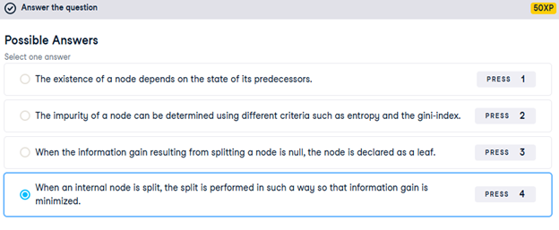
4) Growing a classification tree
In the video, you saw that the growth of an unconstrained classification tree followed a few simple rules. Which of the following is not one of these rules?
5) Using entropy as a criterion
In this exercise, you’ll train a classification tree on the Wisconsin Breast Cancer dataset using entropy as an information criterion. You’ll do so using all the 30 features in the dataset, which is split into 80% train and 20% test.
X_train as well as the array of labels y_train are available in your workspace.
- Import DecisionTreeClassifier from sklearn.tree.
- Instantiate a DecisionTreeClassifier dt_entropy with a maximum depth of 8.
- Set the information criterion to ‘entropy’.
- Fit dt_entropy on the training set.
# Import DecisionTreeClassifier from sklearn.tree
from sklearn.tree import DecisionTreeClassifier
# Instantiate dt_entropy, set ‘entropy’ as the information criterion
dt_entropy = DecisionTreeClassifier(max_depth=8, criterion=’entropy’, random_state=1)
# Fit dt_entropy to the training set
dt_entropy.fit(X_train, y_train)
6) Entropy vs Gini index
In this exercise you’ll compare the test set accuracy of dt_entropy to the accuracy of another tree named dt_gini. The tree dt_gini was trained on the same dataset using the same parameters except for the information criterion which was set to the gini index using the keyword ‘gini’.
X_test, y_test, dt_entropy, as well as accuracy_gini which corresponds to the test set accuracy achieved by dt_gini are available in your workspace.
- Import accuracy_score from sklearn.metrics.
- Predict the test set labels of dt_entropy and assign the result to y_pred.
- Evaluate the test set accuracy of dt_entropy and assign the result to accuracy_entropy.
- Review accuracy_entropy and accuracy_gini.
# Import accuracy_score from sklearn.metrics
from sklearn.metrics import accuracy_score
# Use dt_entropy to predict test set labels
y_pred = dt_entropy.predict(X_test)
# Evaluate accuracy_entropy
accuracy_entropy = accuracy_score(y_test, y_pred)
# Print accuracy_entropy
print(f’Accuracy achieved by using entropy: {accuracy_entropy:.3f}’)
# Print accuracy_gini
print(f’Accuracy achieved by using the gini index: {accuracy_gini:.3f}’)
7) Train your first regression tree
In this exercise, you’ll train a regression tree to predict the mpg (miles per gallon) consumption of cars in the auto-mpg dataset using all the six available features.
The dataset is processed for you and is split to 80% train and 20% test. The features matrix X_train and the array y_train are available in your workspace.
- Import DecisionTreeRegressor from sklearn.tree.
- Instantiate a DecisionTreeRegressor dt with maximum depth 8 and min_samples_leaf set to 0.13.
- Fit dt to the training set.
# Import DecisionTreeRegressor from sklearn.tree
from sklearn.tree import DecisionTreeRegressor
# Instantiate dt
dt = DecisionTreeRegressor(max_depth=8,
min_samples_leaf=0.13,
random_state=3)
# Fit dt to the training set
dt.fit(X_train, y_train)
8) Evaluate the regression tree
In this exercise, you will evaluate the test set performance of dt using the Root Mean Squared Error (RMSE) metric. The RMSE of a model measures, on average, how much the model’s predictions differ from the actual labels. The RMSE of a model can be obtained by computing the square root of the model’s Mean Squared Error (MSE).
The features matrix X_test, the array y_test, as well as the decision tree regressor dt that you trained in the previous exercise are available in your workspace.
- Import the function mean_squared_error as MSE from sklearn.metrics.
- Predict the test set labels and assign the output to y_pred.
- Compute the test set MSE by calling MSE and assign the result to mse_dt.
- Compute the test set RMSE and assign it to rmse_dt.
# Import mean_squared_error from sklearn.metrics as MSE
from sklearn.metrics import mean_squared_error as MSE
# Compute y_pred
y_pred = dt.predict(X_test)
# Compute mse_dt
mse_dt = MSE(y_test, y_pred)
# Compute rmse_dt
rmse_dt = mse_dt**0.5
# Print rmse_dt
print(“Test set RMSE of dt: {:.2f}”.format(rmse_dt))
9) Linear regression vs regression tree
In this exercise, you’ll compare the test set RMSE of dt to that achieved by a linear regression model. We have already instantiated a linear regression model lr and trained it on the same dataset as dt.
The features matrix X_test, the array of labels y_test, the trained linear regression model lr, mean_squared_error function which was imported under the alias MSE and rmse_dt from the previous exercise are available in your workspace.
- Predict test set labels using the linear regression model (lr) and assign the result to y_pred_lr.
- Compute the test set MSE and assign the result to mse_lr.
- Compute the test set RMSE and assign the result to rmse_lr.
# Predict test set labels
y_pred_lr = lr.predict(X_test)
# Compute mse_lr
mse_lr = MSE(y_test, y_pred_lr)
# Compute rmse_lr
rmse_lr = mse_lr**0.5
# Print rmse_lr
print(‘Linear Regression test set RMSE: {:.2f}’.format(rmse_lr))
# Print rmse_dt
print(‘Regression Tree test set RMSE: {:.2f}’.format(rmse_dt))
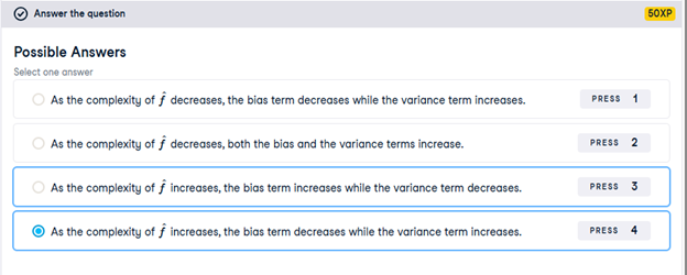
10) Complexity, bias and variance
In the video, you saw how the complexity of a model labeled influences the bias and variance terms of its generalization error.
Which of the following correctly describes the relationship between ‘s complexity and
‘s bias and variance terms?
11) Overfitting and underfitting
In this exercise, you’ll visually diagnose whether a model is overfitting or underfitting the training set.
For this purpose, we have trained two different models and
on the auto dataset to predict the mpg consumption of a car using only the car’s displacement (displ) as a feature.
The following figure shows you scatterplots of mpg versus displ along with lines corresponding to the training set predictions of models and
in red.
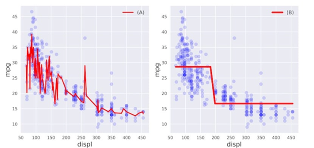
Which of the following statements is true?

12) Instantiate the model
In the following set of exercises, you’ll diagnose the bias and variance problems of a regression tree. The regression tree you’ll define in this exercise will be used to predict the mpg consumption of cars from the auto dataset using all available features.
We have already processed the data and loaded the features matrix X and the array y in your workspace. In addition, the DecisionTreeRegressor class was imported from sklearn.tree.
- Import train_test_split from sklearn.model_selection.
- Split the data into 70% train and 30% test.
- Instantiate a DecisionTreeRegressor with max depth 4 and min_samples_leaf set to 0.26.
# Import train_test_split from sklearn.model_selection
from sklearn.model_selection import train_test_split
# Set SEED for reproducibility
SEED = 1
# Split the data into 70% train and 30% test
X_train, X_test, y_train, y_test = train_test_split(X, y, test_size=0.3, random_state=SEED)
# Instantiate a DecisionTreeRegressor dt
dt = DecisionTreeRegressor(max_depth=4, min_samples_leaf=0.26, random_state=SEED)
13) Evaluate the 10-fold CV error
In this exercise, you’ll evaluate the 10-fold CV Root Mean Squared Error (RMSE) achieved by the regression tree dt that you instantiated in the previous exercise.
In addition to dt, the training data including X_train and y_train are available in your workspace. We also imported cross_val_score from sklearn.model_selection.
Note that since cross_val_score has only the option of evaluating the negative MSEs, its output should be multiplied by negative one to obtain the MSEs. The CV RMSE can then be obtained by computing the square root of the average MSE.
- Compute dt’s 10-fold cross-validated MSE by setting the scoring argument to ‘neg_mean_squared_error’.
- Compute RMSE from the obtained MSE scores.
# Compute the array containing the 10-folds CV MSEs
MSE_CV_scores = – cross_val_score(dt, X_train, y_train,
cv=10,
scoring=’neg_mean_squared_error’,
n_jobs=-1)
# Compute the 10-folds CV RMSE
RMSE_CV = (MSE_CV_scores.mean())**0.5
# Print RMSE_CV
print(‘CV RMSE: {:.2f}’.format(RMSE_CV))
14) Evaluate the training error
You’ll now evaluate the training set RMSE achieved by the regression tree dt that you instantiated in a previous exercise.
In addition to dt, X_train and y_train are available in your workspace.
Note that in scikit-learn, the MSE of a model can be computed as follows:
MSE_model = mean_squared_error(y_true, y_predicted)
where we use the function mean_squared_error from the metrics module and pass it the true labels y_true as a first argument, and the predicted labels from the model y_predicted as a second argument.
- Import mean_squared_error as MSE from sklearn.metrics.
- Fit dt to the training set.
- Predict dt’s training set labels and assign the result to y_pred_train.
- Evaluate dt’s training set RMSE and assign it to RMSE_train.
# Import mean_squared_error from sklearn.metrics as MSE
from sklearn.metrics import mean_squared_error as MSE
# Fit dt to the training set
dt.fit(X_train, y_train)
# Predict the labels of the training set
y_pred_train = dt.predict(X_train)
# Evaluate the training set RMSE of dt
RMSE_train = (MSE(y_train, y_pred_train))**0.5
# Print RMSE_train
print(‘Train RMSE: {:.2f}’.format(RMSE_train))
15) High bias or high variance?
In this exercise you’ll diagnose whether the regression tree dt you trained in the previous exercise suffers from a bias or a variance problem.
The training set RMSE (RMSE_train) and the CV RMSE (RMSE_CV) achieved by dt are available in your workspace. In addition, we have also loaded a variable called baseline_RMSE which corresponds to the root mean-squared error achieved by the regression-tree trained with the disp feature only (it is the RMSE achieved by the regression tree trained in chapter 1, lesson 3). Here baseline_RMSE serves as the baseline RMSE above which a model is considered to be underfitting and below which the model is considered ‘good enough’.
Does dt suffer from a high bias or a high variance problem?

16) Define the ensemble
In the following set of exercises, you’ll work with the Indian Liver Patient Dataset from the UCI Machine learning repository.
In this exercise, you’ll instantiate three classifiers to predict whether a patient suffers from a liver disease using all the features present in the dataset.
The classes LogisticRegression, DecisionTreeClassifier, and KNeighborsClassifier under the alias KNN are available in your workspace.
- Instantiate a Logistic Regression classifier and assign it to lr.
- Instantiate a KNN classifier that considers 27 nearest neighbors and assign it to knn.
- Instantiate a Decision Tree Classifier with the parameter min_samples_leaf set to 0.13 and assign it to dt.
# Set seed for reproducibility
SEED = 1
# Instantiate lr
lr = LogisticRegression(random_state=SEED)
# Instantiate knn
knn = KNN(n_neighbors=27)
# Instantiate dt
dt = DecisionTreeClassifier(min_samples_leaf=0.13, random_state=SEED)
# Define the list classifiers
classifiers = [(‘Logistic Regression’, lr),
(‘K Nearest Neighbours’, knn),
(‘Classification Tree’, dt)]
17) Evaluate individual classifiers
In this exercise you’ll evaluate the performance of the models in the list classifiers that we defined in the previous exercise. You’ll do so by fitting each classifier on the training set and evaluating its test set accuracy.
The dataset is already loaded and preprocessed for you (numerical features are standardized) and it is split into 70% train and 30% test. The features matrices X_train and X_test, as well as the arrays of labels y_train and y_test are available in your workspace. In addition, we have loaded the list classifiers from the previous exercise, as well as the function accuracy_score() from sklearn.metrics.
- Iterate over the tuples in classifiers. Use clf_name and clf as the for loop variables:
- Fit clf to the training set.
- Predict clf’s test set labels and assign the results to y_pred.
- Evaluate the test set accuracy of clf and print the result.
# Iterate over the pre-defined list of classifiers
for clf_name, clf in classifiers:
# Fit clf to the training set
clf.fit(X_train, y_train)
# Predict y_pred
y_pred = clf.predict(X_test)
# Calculate accuracy
accuracy = accuracy_score(y_test, y_pred)
# Evaluate clf’s accuracy on the test set
print(‘{:s} : {:.3f}’.format(clf_name, accuracy))
18) Better performance with a Voting Classifier
Finally, you’ll evaluate the performance of a voting classifier that takes the outputs of the models defined in the list classifiers and assigns labels by majority voting.
X_train, X_test,y_train, y_test, the list classifiers defined in a previous exercise, as well as the function accuracy_score from sklearn.metrics are available in your workspace.
- Import VotingClassifier from sklearn.ensemble.
- Instantiate a VotingClassifier by setting the parameter estimators to classifiers and assign it to vc.
- Fit vc to the training set.
- Evaluate vc’s test set accuracy using the test set predictions y_pred.
# Import VotingClassifier from sklearn.ensemble
from sklearn.ensemble import VotingClassifier
# Instantiate a VotingClassifier vc
vc = VotingClassifier(estimators=classifiers)
# Fit vc to the training set
vc.fit(X_train, y_train)
# Evaluate the test set predictions
y_pred = vc.predict(X_test)
# Calculate accuracy score
accuracy = accuracy_score(y_test, y_pred)
print(‘Voting Classifier: {:.3f}’.format(accuracy))
19) Define the bagging classifier
In the following exercises you’ll work with the Indian Liver Patient dataset from the UCI machine learning repository. Your task is to predict whether a patient suffers from a liver disease using 10 features including Albumin, age and gender. You’ll do so using a Bagging Classifier.
- Import DecisionTreeClassifier from sklearn.tree and BaggingClassifier from sklearn.ensemble.
- Instantiate a DecisionTreeClassifier called dt.
- Instantiate a BaggingClassifier called bc consisting of 50 trees.
# Import DecisionTreeClassifier
from sklearn.tree import DecisionTreeClassifier
# Import BaggingClassifier
from sklearn.ensemble import BaggingClassifier
# Instantiate dt
dt = DecisionTreeClassifier(random_state=1)
# Instantiate bc
bc = BaggingClassifier(base_estimator=dt, n_estimators=50, random_state=1)
20) Evaluate Bagging performance
Now that you instantiated the bagging classifier, it’s time to train it and evaluate its test set accuracy.
The Indian Liver Patient dataset is processed for you and split into 80% train and 20% test. The feature matrices X_train and X_test, as well as the arrays of labels y_train and y_test are available in your workspace. In addition, we have also loaded the bagging classifier bc that you instantiated in the previous exercise and the function accuracy_score() from sklearn.metrics.
- Fit bc to the training set.
- Predict the test set labels and assign the result to y_pred.
- Determine bc’s test set accuracy.
# Fit bc to the training set
bc.fit(X_train, y_train)
# Predict test set labels
y_pred = bc.predict(X_test)
# Evaluate acc_test
acc_test = accuracy_score(y_test, y_pred)
print(‘Test set accuracy of bc: {:.2f}’.format(acc_test))
21) Prepare the ground
In the following exercises, you’ll compare the OOB accuracy to the test set accuracy of a bagging classifier trained on the Indian Liver Patient dataset.
In sklearn, you can evaluate the OOB accuracy of an ensemble classifier by setting the parameter oob_score to True during instantiation. After training the classifier, the OOB accuracy can be obtained by accessing the .oob_score_ attribute from the corresponding instance.
In your environment, we have made available the class DecisionTreeClassifier from sklearn.tree.
- Import BaggingClassifier from sklearn.ensemble.
- Instantiate a DecisionTreeClassifier with min_samples_leaf set to 8.
- Instantiate a BaggingClassifier consisting of 50 trees and set oob_score to True.
# Import DecisionTreeClassifier
from sklearn.tree import DecisionTreeClassifier
# Import BaggingClassifier
from sklearn.ensemble import BaggingClassifier
# Instantiate dt
dt = DecisionTreeClassifier(min_samples_leaf=8, random_state=1)
# Instantiate bc
bc = BaggingClassifier(base_estimator=dt,
n_estimators=50,
oob_score=True,
random_state=1)
22) OOB Score vs Test Set Score
Now that you instantiated bc, you will fit it to the training set and evaluate its test set and OOB accuracies.
The dataset is processed for you and split into 80% train and 20% test. The feature matrices X_train and X_test, as well as the arrays of labels y_train and y_test are available in your workspace. In addition, we have also loaded the classifier bc instantiated in the previous exercise and the function accuracy_score() from sklearn.metrics.
- Fit bc to the training set and predict the test set labels and assign the results to y_pred.
- Evaluate the test set accuracy acc_test by calling accuracy_score.
- Evaluate bc’s OOB accuracy acc_oob by extracting the attribute oob_score_ from bc.
# Fit bc to the training set
bc.fit(X_train, y_train)
# Predict test set labels
y_pred = bc.predict(X_test)
# Evaluate test set accuracy
acc_test = accuracy_score(y_test, y_pred)
# Evaluate OOB accuracy
acc_oob = bc.oob_score_
# Print acc_test and acc_oob
print(‘Test set accuracy: {:.3f}, OOB accuracy: {:.3f}’.format(acc_test, acc_oob))
23) Train an RF regressor
In the following exercises you’ll predict bike rental demand in the Capital Bikeshare program in Washington, D.C using historical weather data from the Bike Sharing Demand dataset available through Kaggle. For this purpose, you will be using the random forests algorithm. As a first step, you’ll define a random forests regressor and fit it to the training set.
The dataset is processed for you and split into 80% train and 20% test. The features matrix X_train and the array y_train are available in your workspace.
- Import RandomForestRegressor from sklearn.ensemble.
- Instantiate a RandomForestRegressor called rf consisting of 25 trees.
- Fit rf to the training set.
# Import RandomForestRegressor
from sklearn.ensemble import RandomForestRegressor
# Instantiate rf
rf = RandomForestRegressor(n_estimators=25,
random_state=2)
# Fit rf to the training set
rf.fit(X_train, y_train)
24) Evaluate the RF regressor
You’ll now evaluate the test set RMSE of the random forests regressor rf that you trained in the previous exercise.
The dataset is processed for you and split into 80% train and 20% test. The features matrix X_test, as well as the array y_test are available in your workspace. In addition, we have also loaded the model rf that you trained in the previous exercise.
- Import mean_squared_error from sklearn.metrics as MSE.
- Predict the test set labels and assign the result to y_pred.
- Compute the test set RMSE and assign it to rmse_test.
# Import mean_squared_error as MSE
from sklearn.metrics import mean_squared_error as MSE
# Predict the test set labels
y_pred = rf.predict(X_test)
# Evaluate the test set RMSE
rmse_test = (MSE(y_test, y_pred))**0.5
# Print rmse_test
print(‘Test set RMSE of rf: {:.2f}’.format(rmse_test))
25) Visualizing features importances
In this exercise, you’ll determine which features were the most predictive according to the random forests regressor rf that you trained in a previous exercise.
For this purpose, you’ll draw a horizontal barplot of the feature importance as assessed by rf. Fortunately, this can be done easily thanks to plotting capabilities of pandas.
We have created a pandas.Series object called importances containing the feature names as index and their importances as values. In addition, matplotlib.pyplot is available as plt and pandas as pd.
- Call the .sort_values() method on importances and assign the result to importances_sorted.
- Call the .plot() method on importances_sorted and set the arguments:
- kind to ‘barh’
- color to ‘lightgreen’
# Create a pd.Series of features importances
importances = pd.Series(data=rf.feature_importances_,
index=X_train.columns)
# Sort importances
importances_sorted = importances.sort_values()
# Draw a horizontal barplot of importances_sorted
importances_sorted.plot(kind=’barh’, color=’lightgreen’)
plt.title(‘Features Importances’)
plt.show()
26) Define the AdaBoost classifier
In the following exercises you’ll revisit the Indian Liver Patient dataset which was introduced in a previous chapter. Your task is to predict whether a patient suffers from a liver disease using 10 features including Albumin, age and gender. However, this time, you’ll be training an AdaBoost ensemble to perform the classification task. In addition, given that this dataset is imbalanced, you’ll be using the ROC AUC score as a metric instead of accuracy.
As a first step, you’ll start by instantiating an AdaBoost classifier.
- Import AdaBoostClassifier from sklearn.ensemble.
- Instantiate a DecisionTreeClassifier with max_depth set to 2.
- Instantiate an AdaBoostClassifier consisting of 180 trees and setting the base_estimator to dt.
# Import DecisionTreeClassifier
from sklearn.tree import DecisionTreeClassifier
# Import AdaBoostClassifier
from sklearn.ensemble import AdaBoostClassifier
# Instantiate dt
dt = DecisionTreeClassifier(max_depth=2, random_state=1)
# Instantiate ada
ada = AdaBoostClassifier(base_estimator=dt, n_estimators=180, random_state=1)
27) Train the AdaBoost classifier
Now that you’ve instantiated the AdaBoost classifier ada, it’s time train it. You will also predict the probabilities of obtaining the positive class in the test set. This can be done as follows:
Once the classifier ada is trained, call the .predict_proba() method by passing X_test as a parameter and extract these probabilities by slicing all the values in the second column as follows:
ada.predict_proba(X_test)[:,1]
The Indian Liver dataset is processed for you and split into 80% train and 20% test. Feature matrices X_train and X_test, as well as the arrays of labels y_train and y_test are available in your workspace. In addition, we have also loaded the instantiated model ada from the previous exercise.
- Fit ada to the training set.
- Evaluate the probabilities of obtaining the positive class in the test set.
# Fit ada to the training set
ada.fit(X_train, y_train)
# Compute the probabilities of obtaining the positive class
y_pred_proba = ada.predict_proba(X_test)[:, 1]
28) Evaluate the AdaBoost classifier
Now that you’re done training ada and predicting the probabilities of obtaining the positive class in the test set, it’s time to evaluate ada’s ROC AUC score. Recall that the ROC AUC score of a binary classifier can be determined using the roc_auc_score() function from sklearn.metrics.
The arrays y_test and y_pred_proba that you computed in the previous exercise are available in your workspace.
- Import roc_auc_score from sklearn.metrics.
- Compute ada’s test set ROC AUC score, assign it to ada_roc_auc, and print it out.
# Import roc_auc_score
from sklearn.metrics import roc_auc_score
# Evaluate test-set roc_auc_score
ada_roc_auc = roc_auc_score(y_test, y_pred_proba)
# Print roc_auc_score
print(‘ROC AUC score: {:.2f}’.format(ada_roc_auc))
29) Define the GB regressor
You’ll now revisit the Bike Sharing Demand dataset that was introduced in the previous chapter. Recall that your task is to predict the bike rental demand using historical weather data from the Capital Bikeshare program in Washington, D.C.. For this purpose, you’ll be using a gradient boosting regressor.
As a first step, you’ll start by instantiating a gradient boosting regressor which you will train in the next exercise.
- Import GradientBoostingRegressor from sklearn.ensemble.
- Instantiate a gradient boosting regressor by setting the parameters:
- max_depth to 4
- n_estimators to 200
# Import GradientBoostingRegressor
from sklearn.ensemble import GradientBoostingRegressor
# Instantiate gb
gb = GradientBoostingRegressor(max_depth=4,
n_estimators=200,
random_state=2)
30) Train the GB regressor
You’ll now train the gradient boosting regressor gb that you instantiated in the previous exercise and predict test set labels.
The dataset is split into 80% train and 20% test. Feature matrices X_train and X_test, as well as the arrays y_train and y_test are available in your workspace. In addition, we have also loaded the model instance gb that you defined in the previous exercise.
- Fit gb to the training set.
- Predict the test set labels and assign the result to y_pred.
# Fit gb to the training set
gb.fit(X_train, y_train)
# Predict test set labels
y_pred = gb.predict(X_test)
31) Evaluate the GB regressor
Now that the test set predictions are available, you can use them to evaluate the test set Root Mean Squared Error (RMSE) of gb.
y_test and predictions y_pred are available in your workspace.
- Import mean_squared_error from sklearn.metrics as MSE.
- Compute the test set MSE and assign it to mse_test.
- Compute the test set RMSE and assign it to rmse_test.
# Import mean_squared_error as MSE
from sklearn.metrics import mean_squared_error as MSE
# Compute MSE
mse_test = MSE(y_test, y_pred)
# Compute RMSE
rmse_test = mse_test ** 0.5
# Print RMSE
print(‘Test set RMSE of gb: {:.3f}’.format(rmse_test))
32) Regression with SGB
As in the exercises from the previous lesson, you’ll be working with the Bike Sharing Demand dataset. In the following set of exercises, you’ll solve this bike count regression problem using stochastic gradient boosting.
- Instantiate a Stochastic Gradient Boosting Regressor (SGBR) and set:
- max_depth to 4 and n_estimators to 200,
- subsample to 0.9, and
- max_features to 0.75.
# Import GradientBoostingRegressor
from sklearn.ensemble import GradientBoostingRegressor
# Instantiate sgbr
sgbr = GradientBoostingRegressor(max_depth=4,
subsample=0.9,
max_features=0.75,
n_estimators=200,
random_state=2)
33) Train the SGB regressor
In this exercise, you’ll train the SGBR sgbr instantiated in the previous exercise and predict the test set labels.
The bike sharing demand dataset is already loaded processed for you; it is split into 80% train and 20% test. The feature matrices X_train and X_test, the arrays of labels y_train and y_test, and the model instance sgbr that you defined in the previous exercise are available in your workspace.
- Fit sgbr to the training set.
- Predict the test set labels and assign the results to y_pred.
# Fit sgbr to the training set
sgbr.fit(X_train, y_train)
# Predict test set labels
y_pred = sgbr.predict(X_test)
34) Evaluate the SGB regressor
You have prepared the ground to determine the test set RMSE of sgbr which you shall evaluate in this exercise.
y_pred and y_test are available in your workspace.
- Import mean_squared_error as MSE from sklearn.metrics.
- Compute test set MSE and assign the result to mse_test.
- Compute test set RMSE and assign the result to rmse_test.
# Import mean_squared_error as MSE
from sklearn.metrics import mean_squared_error as MSE
# Compute test set MSE
mse_test = MSE(y_test, y_pred)
# Compute test set RMSE
rmse_test = mse_test ** 0.5
# Print rmse_test
print(‘Test set RMSE of sgbr: {:.3f}’.format(rmse_test))
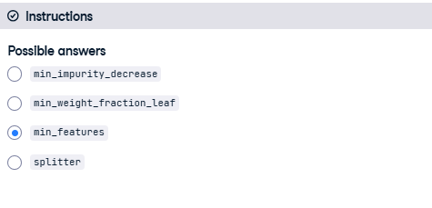
35) Tree hyperparameters
In the following exercises you’ll revisit the Indian Liver Patient dataset which was introduced in a previous chapter.
Your task is to tune the hyperparameters of a classification tree. Given that this dataset is imbalanced, you’ll be using the ROC AUC score as a metric instead of accuracy.
We have instantiated a DecisionTreeClassifier and assigned to dt with sklearn’s default hyperparameters. You can inspect the hyperparameters of dt in your console.
Which of the following is not a hyperparameter of dt?
36) Set the tree’s hyperparameter grid
In this exercise, you’ll manually set the grid of hyperparameters that will be used to tune the classification tree dt and find the optimal classifier in the next exercise.
- Define a grid of hyperparameters corresponding to a Python dictionary called params_dt with:
- the key ‘max_depth’ set to a list of values 2, 3, and 4
- the key ‘min_samples_leaf’ set to a list of values 0.12, 0.14, 0.16, 0.18
# Define params_dt
params_dt = {
‘max_depth’: [2, 3, 4],
‘min_samples_leaf’: [0.12, 0.14, 0.16, 0.18]
}
37) Search for the optimal tree
In this exercise, you’ll perform grid search using 5-fold cross validation to find dt’s optimal hyperparameters. Note that because grid search is an exhaustive process, it may take a lot time to train the model. Here you’ll only be instantiating the GridSearchCV object without fitting it to the training set. As discussed in the video, you can train such an object similar to any scikit-learn estimator by using the .fit() method:
grid_object.fit(X_train, y_train)
An untuned classification tree dt as well as the dictionary params_dt that you defined in the previous exercise are available in your workspace.
- Import GridSearchCV from sklearn.model_selection.
- Instantiate a GridSearchCV object using 5-fold CV by setting the parameters:
- estimator to dt, param_grid to params_dt and
- scoring to ‘roc_auc’.
# Import GridSearchCV
from sklearn.model_selection import GridSearchCV
# Instantiate grid_dt
grid_dt = GridSearchCV(estimator=dt,
param_grid=params_dt,
scoring=’roc_auc’,
cv=5,
n_jobs=-1)
38) Evaluate the optimal tree
In this exercise, you’ll evaluate the test set ROC AUC score of grid_dt’s optimal model.
In order to do so, you will first determine the probability of obtaining the positive label for each test set observation. You can use the methodpredict_proba() of an sklearn classifier to compute a 2D array containing the probabilities of the negative and positive class-labels respectively along columns.
The dataset is already loaded and processed for you (numerical features are standardized); it is split into 80% train and 20% test. X_test, y_test are available in your workspace. In addition, we have also loaded the trained GridSearchCV object grid_dt that you instantiated in the previous exercise. Note that grid_dt was trained as follows:
- Import roc_auc_score from sklearn.metrics.
- Extract the .best_estimator_ attribute from grid_dt and assign it to best_model.
- Predict the test set probabilities of obtaining the positive class y_pred_proba.
- Compute the test set ROC AUC score test_roc_auc of best_model.
# Import roc_auc_score from sklearn.metrics
from sklearn.metrics import roc_auc_score
# Extract the best estimator
best_model = grid_dt.best_estimator_
# Predict the test set probabilities of the positive class
y_pred_proba = best_model.predict_proba(X_test)[:, 1]
# Compute test_roc_auc
test_roc_auc = roc_auc_score(y_test, y_pred_proba)
# Print test_roc_auc
print(‘Test set ROC AUC score: {:.3f}’.format(test_roc_auc))
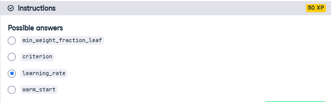
39) Random forests hyperparameters
In the following exercises, you’ll be revisiting the Bike Sharing Demand dataset that was introduced in a previous chapter. Recall that your task is to predict the bike rental demand using historical weather data from the Capital Bikeshare program in Washington, D.C.. For this purpose, you’ll be tuning the hyperparameters of a Random Forests regressor.
We have instantiated a RandomForestRegressor called rf using sklearn’s default hyperparameters. You can inspect the hyperparameters of rf in your console.
Which of the following is not a hyperparameter of rf?
40) Set the hyperparameter grid of RF
In this exercise, you’ll manually set the grid of hyperparameters that will be used to tune rf’s hyperparameters and find the optimal regressor. For this purpose, you will be constructing a grid of hyperparameters and tune the number of estimators, the maximum number of features used when splitting each node and the minimum number of samples (or fraction) per leaf.
- Define a grid of hyperparameters corresponding to a Python dictionary called params_rf with:
- the key ‘n_estimators’ set to a list of values 100, 350, 500
- the key ‘max_features’ set to a list of values ‘log2’, ‘auto’, ‘sqrt’
- the key ‘min_samples_leaf’ set to a list of values 2, 10, 30
# Define the dictionary ‘params_rf’
params_rf = {
‘n_estimators’: [100, 350, 500],
‘max_features’: [‘log2’, ‘auto’, ‘sqrt’],
‘min_samples_leaf’: [2, 10, 30]
}
41) Search for the optimal forest
In this exercise, you’ll perform grid search using 3-fold cross validation to find rf’s optimal hyperparameters. To evaluate each model in the grid, you’ll be using the negative mean squared error metric.
Note that because grid search is an exhaustive search process, it may take a lot time to train the model. Here you’ll only be instantiating the GridSearchCV object without fitting it to the training set. As discussed in the video, you can train such an object similar to any scikit-learn estimator by using the .fit() method:
grid_object.fit(X_train, y_train)
The untuned random forests regressor model rf as well as the dictionary params_rf that you defined in the previous exercise are available in your workspace.
- Import GridSearchCV from sklearn.model_selection.
- Instantiate a GridSearchCV object using 3-fold CV by using negative mean squared error as the scoring metric.
# Import GridSearchCV
from sklearn.model_selection import GridSearchCV
# Instantiate grid_rf
grid_rf = GridSearchCV(estimator=rf,
param_grid=params_rf,
scoring=’neg_mean_squared_error’,
cv=3,
verbose=1,
n_jobs=-1)
42) Evaluate the optimal forest
In this last exercise of the course, you’ll evaluate the test set RMSE of grid_rf’s optimal model.
The dataset is already loaded and processed for you and is split into 80% train and 20% test. In your environment are available X_test, y_test and the function mean_squared_error from sklearn.metrics under the alias MSE. In addition, we have also loaded the trained GridSearchCV object grid_rf that you instantiated in the previous exercise. Note that grid_rf was trained as follows:
grid_rf.fit(X_train, y_train)
- Import mean_squared_error as MSE from sklearn.metrics.
- Extract the best estimator from grid_rf and assign it to best_model.
- Predict best_model’s test set labels and assign the result to y_pred.
- Compute best_model’s test set RMSE.
# Import mean_squared_error from sklearn.metrics as MSE
from sklearn.metrics import mean_squared_error as MSE
# Extract the best estimator
best_model = grid_rf.best_estimator_
# Predict test set labels
y_pred = best_model.predict(X_test)
# Compute rmse_test
rmse_test = (MSE(y_test, y_pred))**0.5
# Print rmse_test
print(‘Test RMSE of best model: {:.3f}’.format(rmse_test))